12.4 – ANOVA from “sufficient statistics”
Introduction
By now you should be able to run a one-way ANOVA using R (and R Commander) with ease. As a reminder, You should also be aware that, if you need to, you could use spreadsheet software like Microsoft Excel or LibreOffice Calc to run one way ANOVA on a small data set. Still, there are times when you may need to run a one-way ANOVA on a small data set, and doing so by hand calculator may be just as convenient. What are your available options?
Following the formulas I have given would be one way to calculate ANOVA by hand, but it would be tedious and subject to error. Instead of working with the standard formulas, calculator shortcuts can be derived with a little algebra and this is where I want to draw your attention now. This technique will come in handy in lab classes or other scenarios where you collect some data among a set number of groups and calculate means and standard deviations. The purpose of this posting is to show you how to obtain the necessary statistics to calculate a one-way ANOVA from the available descriptive statistics: means, standard deviations, and sample sizes. In other words, these are the sufficient statistics for one-way ANOVA.
Note in Chapter 11.5, we introduced use of summary statistics, i.e., “sufficient statistics,” to calculate the independent sample t-test.
As you recall, a one-way ANOVA yields a single F test of the null hypothesis that all group means are equal. To calculate the F test, you need
- Mean Square Between Groups,

- Mean Squares Within Groups or Error,

F is then calculated as

with degrees of freedom k – 1 for the numerator and N – 1 for the denominator. can also appear as 
We can calculate as

where k is the number of i th groups, ni is the sample size of the ith group,  refers to the overall mean for all of the
  sample means.
Next, for the Error Mean Square, , all we need is the average of the sample variances (the square of the sample standard deviation, s).

ANOVA from sufficient statistics
Consider an example data set (Table 1) for which only summary statistics are available (mean and standard deviation, sd). The data set is for metabolic rate (ml oxygen per hour) for strains of laboratory mice. Sample size for each group was seven mice.
Table 1. Descriptive statistics wheel-running behavior mice from ten different inbred strains of mice (Mus domesticus).
| Strain | n | Mean | sd |
| AKR | 7 | 395 | 169.7 |
| C57BL_10 | 7 | 1135 | 63.6 |
| CBA | 7 | 855 | 77.8 |
| 129S1 | 7 | 1012 | 176.8 |
| C3H/He | 7 | 833 | 49.5 |
| C57BL/6 | 7 | 1075 | 91.9 |
| FVB/N | 7 | 1023 | 91.9 |
| A | 7 | 806 | 134.4 |
| BALB/c | 7 | 936 | 70.7 |
| DBA/2 | 7 | 872 | 49.5 |
Spreadsheet calculations
You have several options at this point, ranging from using your calculator and the formulas above (don’t forget to square the standard deviation to get the variances!), or you could use Microsoft Excel or LibreOffice Calc and enter the necessary formulas by hand (Table 2). You’ll also find many online calculators for one-way ANOVA by sufficient statistics (e.g., https://www.danielsoper.com/statcalc/calculator.aspx?id=43).
Table 2. Spreadsheet with formulas for calculating one-way ANOVA from means and standard deviations from statistics presented in Table 1.
| A | B | C | D | E | F | G | H | I | |
| 1 | Strain | n | Mean | sd | squared | variance | grand mean |
=AVERAGE(C:C) | |
| 2 | AKR | 7 | 395 | 169.7 | =B2*(C2-$I$1)^2 | =D2^2 | dfB | =COUNT(B:B)-1 | |
| 3 | C57BL_10 | 7 | 1135 | 63.6 | =B2*(C3-$I$1)^2 | =D3^2 | dfE | =SUM(B:B)-I2 | |
| 4 | CBA | 7 | 855 | 77.8 | =B2*(C4-$I$1)^2 | =D4^2 | Msb | =SUM(E:E)/(COUNT(E:E)-1) | |
| 5 | 129S1 | 7 | 1012 | 176.8 | =B2*(C5-$I$1)^2 | =D5^2 | Mse | =SUM(F:F)/COUNT(F:F) | |
| 6 | C3H/He | 7 | 833 | 49.5 | =B2*(C6-$I$1)^2 | =D6^2 | F | =I4/I5 | |
| 7 | C57BL/6 | 7 | 1075 | 91.9 | =B2*(C7-$I$1)^2 | =D7^2 | P-value | =FDIST(I6,I2,I3) | |
| 8 | FVB/N | 7 | 1023 | 91.9 | =B2*(C8-$I$1)^2 | =D8^2 | |||
| 9 | A | 7 | 806 | 134.4 | =B2*(C9-$I$1)^2 | =D9^2 | |||
| 10 | BALB/c | 7 | 936 | 70.7 | =B2*(C10-$I$1)^2 | =D10^2 | |||
| 11 | DBA/2 | 7 | 872 | 49.5 | =B2*(C11-$I$1)^2 | =D11^2 |
For this example, you should get the following
MSB = 299943.5

MSE = 11500.8

F = 26.08

P-value = 9.75E-18
Note: The number of figures reported for the P-value implies a precision that the data simply do not support. For a report, recommend writing the P-value < 0.001
But, R can do it better.
Here’s how. Install the HH package (or RcmdrPlugin.HH for use in Rcmdr) and call the aovSufficient function.
Step 1. Install the HH package from a CRAN mirror, e.g., cloud.r-project.org, in the usual way.
chooseCRANmirror()
install.packages("HH")
library(HH)
Step 2. Enter the data. Do this in the usual way (e.g., from a text file), or enter directly using the read.table command as follows.
MouseData <- read.table(header=TRUE, sep = "", text=
"Strain Mean sd
AKR 395 169.7
C57BL_10 1135 63.6
CBA 855 77.8
129S1 1012 176.8
C3H/He 833 49.5
C57BL/6 1075 91.9
FVB/N 1023 91.9
A 806 134.4
BALB/c 936 70.7
DBA/2 872 49.5")
#Check import
head(MouseData)
End of R input
I know, a little hard to read, but from the MouseData to the end bracket “) before the comment line #Check import, that’s all one command.
Of course, you could copy the data and import the data from your computer’s clipboard in Rcmdr: Data → Import data → from text file, clipboard, or URL… (Hint: for field separator, try White space; if that fails, try Tabs).
Once the data set is loaded, proceed to Step 3.
Step 3. In our example, sample size is included for each group. Skip to step 4. If, however, the table lacked the sample size information, you can always add a new variable. For example, if we needed to add sample size to the data frame, we would use the repeat element function, rep().
MouseData$n <- rep(7, 10)
If you check the View data set button in Rcmdr, you will see that the command in Step 3 has added a new variable “n” for each of the eleven rows. The function rep() stands for “replicate elements in vectors” and what it did here was enter a value of 7 for each of the ten rows in the data set. Again, this step is not necessary for this example because sample size is already part of the data frame. Proceed to step 4.
Step 4. Run the one way ANOVA using the sufficient statistics and the HH function aovSufficient
MouseData.aov <- aovSufficient(Mean ~ Strain, data=MouseData)
Step 5. Get the ANOVA table
summary(MouseData.aov)
Here’s the R output
            Df  Sum Sq  Mean Sq  F value  Pr(>F)
Strain       9 2699491   299943    26.08  <2e-16 ***
Residuals   60  690046    11501
----
Signif. codes:  0 '***' 0.001 '**' 0.01 '*' 0.05 '.' 0.1 ' ' 1
End R output
To explore other features of the package, type ?aovSufficient at the R prompt (like all R functions, extensive help is generally available for each function in a package).
Limitations of ANOVA from sufficient statistics
This was pretty easy, so it is worth asking — Why go through the bother of analyzing the raw data, why not just go to the summary statistics and run the calculator formula? First, the chief reason against the calculator formula and use of only sufficient statistics loses information about the individual values and therefore you have no access to the residuals. The residual of an observation is the difference between the original observation and the model prediction. The residuals are important for determining whether the model fits the data well and are, therefore, part of the toolkit that statisticians need to do proper data analysis. We will spend considerable time looking at residual patterns and it is an important aspect of doing statistics correctly.
Secondly, while it is possible to extend this approach to more complicated ANOVA problems like the two-way ANOVA (Cohen 2002), the statistical significance of the interaction term(s) calculated in this way are only approximate (the main effects are OK to interpret). Thus, ANOVA from sufficient statistics has its place when all you have is access to descriptive statistics, but its use is limited and not at all the preferred option for data analysis when the original, raw observations are in hand.
Questions
1. Under what circumstances would you use “sufficient statistics” to calculate a one-way ANOVA?
2. Calculate the one-way ANOVA for body weight of 47 female (F) and 97 male (M) cats (kilograms, dataset cats in MASS R package) from the following summary statistics.
| n | Mean | sd | |
| F | 47 | 2.36 | 0.274 |
| M | 97 | 2.9 | 0.468 |
3. Bonus: Load the cats data set (package MASS, loaded with Rcmdr) and run a one-way ANOVA using the aov() function via Rcmdr. Are the ANOVA from sufficient statistics the same as results from the direct ANOVA calculation? If not, why not.
Chapter 12 contents
7.4 – Epidemiology: Relative risk and absolute risk, explained
Introduction
Epidemiology is the study of patterns of health and illness of populations. An important task in an epidemiology study is to identify risks associated with disease. Epidemiology is a crucial discipline used to inform about possible effective treatment approaches, health policy, and about the etiology of disease.
Please review terms presented in section 7.1 before proceeding. RR and AR are appropriate for cohort-control and cross-sectional studies (see 2.4 and 5.4) where base rates of exposure and unexposed or numbers of affected and non-affected individuals (prevalence) are available. Calculations of relative risk (RR) and relative risk reduction (RRR) are specific to the sampled groups under study whereas absolute risk (AR) and absolute risk reduction (ARR) pertain to the reference population. Relative risks are specific to the study, absolute risks are generalized to the population. Number needed to treat (NNT) is a way to communicate absolute risk reductions.
An example of ARR and RRR risk calculations using natural numbers
Clinical trials are perhaps the essential research approach (Sibbald and Roland 1998; Sylvester et al 2017); they are often characterized with a binary outcome. Subjects either get better or they do not. There are many ways to represent risk of a particular outcome, but where possible, using natural numbers is generally preferred as a means of communication. Consider the following example (pp 34-35, Gigerenzer 2015): What is the benefit of taking a cholesterol-lowering drug, Pravastatin, on the risk of deaths by heart attacks and other causes of mortality\? Press releases (e.g., Maugh 1995), from the study stated the following:
“… the drug pravastatin reduced … deaths from all causes 22%”
A subsequent report (Skolbekken 1998) presented the following numbers (Table 1).
Table 1. Reduction in total mortality (5 year study) for people who took Pravastatin compared to those who took placebo.
| Deaths per 1000 people with high cholesterol (> 240 mg/dL) |
No deaths | Cumulative incidence |
||
| Treatment | Pravastatin
(n = 3302) |
a= 32 |
b= 3270 |
CIe |
| Placebo
(n = 3293) |
c= 41 |
d= 3252 |
CIu | |
where cumulative incidence refers to the number of new events or cases of disease divided by the total number of individuals in the population at risk.
Do the calculations of risk
The risk reduction (RR), or the number of people who die without treatment (placebo) minus those who die with treatment (Pravastatin), 

and the cumulative incidence in the exposed (treated) group, CIe, is  , and cumulative incidence in the unexposed (control) group, CIu, is
  . We can calculate another statistic called the risk ratio,

because the risk ratio is less than one, we interpret that statins reduce the risk of mortality from heart attack. In other words, statins lowered the risk by 0.78.
But is this risk reduction meaningful?
Now, consider the absolute risk reduction (ARR) is 
Relative risk reduction, or the absolute risk reduction divided by the proportion of patients who die without treatment, is 
Conclusion: high cholesterol may contribute to increased risk of mortality, but the rate is very low in the population as a whole (the ARR).
Another useful way to communicate benefit is to calculate the Number Needed to Treat (NNT), or the number of people who must receive the treatment to save (benefit) one person. The ideal NNT is a value of one (1), which would be interpreted as everyone improves who receives the treatment. By definition, NNT must be positive; however, a resulting negative NNT would suggest the treatment may cause harm, i.e., number needed to harm (NNH).
For this example, the NNT is

therefore, to benefit one person, 111 need to be treated. The flip side of the implications of NNT, although one person may benefit by taking the treatment, 110 ( ) will take the treatment, but will NOT RECEIVE THE BENEFIT, but do potentially get any side effect of the treatment.
Confidence interval for NNT is derived from the Confidence interval for ARR
For a sample of 100 people drawn at random from a population (which may number in the millions), then repeat the NNT calculation for a different sample of 100 people, do we expect the first and second NNT estimates to be exactly the same number\? No, but we do expect them to be close and we can define what we mean by close as we expect each estimate to be within certain limits. While we expect the second calculation to be close to the first estimate, we would be surprised if it was exactly the same. And so, which is the correct estimate, the first or the second\? They both are, in the sense that they both estimate the parameter NNT (a property of a population).
We use confidence interval to communicate where we believe the true estimate for NNT to be. Confidence Intervals (CI) allow us to assign a probability to how certain we are about the statistic and whether it is likely to be close to the true value (Altman 1998, Bender 2001). We will calculate the 95% CI for the ARR using the Wald method, then take the inverse of these estimates for our 95% CI. The Wald method assumes normality.
For CI of ARR, we need sample size for control and treatment groups; like all confidence intervals, we need to calculate the standard error of the statistic, in this, case, the standard error (SE) for ARR is approximately

where SE is the standard error for ARR. For our example, we have

The 95% CI for ARR is approximately 
For the Wald estimate, replace the 2 with  , which comes from the normal table for z at
(why the 2 in the equation? Because it is plus or minus so we divide the frequency 0.95 in half) and for our example, we have 
and the inverse for NNT CI is 
Our example exemplifies the limitation of the Wald approach (cf. Altman 1998): our confidence interval includes zero, and doesn’t even include our best estimate of NNT (111).
Note 1: By now I trust you can see differences for results by direct input of the numbers into R and what you get by the natural numbers approach. In part this is because we round in our natural number calculations — remember, while it makes more sense to communicate about whole numbers (people) and not fractions (fractions of people!), rounding through the calculations adds error to the final value. As long as you know the difference and the relevance between approximate and exact solutions, this shouldn’t cause concern.
Software: epiR
R has many epidemiology packages, epiR and epitools are two. Most of the code presented stems from epiR.
We need to know about our study design in order to tell the functions which statistics are appropriate to estimate. For our statin example, the design was prospective cohort (i.e., cohort.count in epiR package language), not case-control or cross-sectional (review in Chapter 5.4).
library(epiR)
Table1 <- matrix(c(32,3270,41,3252), 2, 2, byrow=TRUE, dimnames = list(c("Statin", "Placebo"), c("Died", "Lived")))
Table1
        Died Lived
Statin    32  3270
Placebo   41  3252
epi.2by2(Table1, method="cohort.count", outcome = "as.columns")
R output
           Outcome + Outcome - Total           Inc risk *
Exposed +         32      3270  3302 0.97  (0.66 to 1.37)
Exposed -         41      3252  3293 1.25  (0.89 to 1.69)
Total             73      6522  6595 1.11  (0.87 to 1.39)

Point estimates and 95% CIs:
-------------------------------------------------------------------
Inc risk ratio                          0.78 (0.49, 1.23)
Inc odds ratio                          0.78 (0.49, 1.24)
Attrib risk in the exposed *           -0.28 (-0.78, 0.23)
Attrib fraction in the exposed (%)    -28.48 (-103.47, 18.88)
Attrib risk in the population *        -0.14 (-0.59, 0.32)
Attrib fraction in the population (%) -12.48 (-37.60, 8.05)
-------------------------------------------------------------------
Uncorrected chi2 test that OR = 1: chi2(1) = 1.147 Pr>chi2 = 0.284
Fisher exact test that OR = 1: Pr>chi2 = 0.292
Wald confidence limits
CI: confidence interval
* Outcomes per 100 population units
The risk ratio we calculated by hand is shown in green in the R output, along with other useful statistics (see \?epi2x2 for help with these additional terms) not defined in our presentation.
We explain results of chi-square goodness of fit (Ch 9.1) and Fisher exact (Ch 9.5) tests in Chapter 9. Suffice to say here, we interpret the p-value (Pr) = 0.284 and 0.292 to indicate that there is no association between mortality from heart attacks with or without the statin (i.e., the Odds Ratio, OR, not statistically different from one).
Wait! Where’s NNT and other results\?
Use another command in epiR package, epi.tests(), to determine the specificity, sensitivity, and positive (or negative) predictive value.
epi.tests(Table1)
and R returns
          Outcome + Outcome - Total
Test +           32      3270  3302
Test -           41      3252  3293
Total            73      6522  6595

Point estimates and 95% CIs:
--------------------------------------------------------------
Apparent prevalence *                    0.50 (0.49, 0.51)
True prevalence *                        0.01 (0.01, 0.01)
Sensitivity *                            0.44 (0.32, 0.56)
Specificity *                            0.50 (0.49, 0.51)
Positive predictive value *              0.01 (0.01, 0.01)
Negative predictive value *              0.99 (0.98, 0.99)
Positive likelihood ratio                0.87 (0.67, 1.13)
Negative likelihood ratio                1.13 (0.92, 1.38)
False T+ proportion for true D- *        0.50 (0.49, 0.51)
False T- proportion for true D+ *        0.56 (0.44, 0.68)
False T+ proportion for T+ *             0.99 (0.99, 0.99)
False T- proportion for T- *             0.01 (0.01, 0.02)
Correctly classified proportion *        0.50 (0.49, 0.51)
--------------------------------------------------------------
* Exact CIs
Additional statistics are available by saving the output from epi2x2() or epitests() to an object, then using summary(). For example save output from epi.2by2(Table1, method="cohort.count", outcome = "as.columns") to object myEpi, then
summary(myEpi)
look for NNT in the R output
$massoc.detail$NNT.strata.wald
       est    lower    upper
1 -362.377 -128.038  436.481
Thus, the NNT was 362 (compared to 111 we got by hand) with 95% Confidence interval between -436 and +128 (make it positive because it is a treatment improvement.)
Note 2: Strata (L. layers), refer to subgroups, for example, sex or age categories (see discussion in Ch05.4). Our examples here are not presented as subgroup analysis, but epiR reports by name strata.
epiR reports a lot of additional statistics in the output and for clarity, I have not defined each one, just the basic terms we need for BI311. As always, see help pages (e.g., \?epi.2x2 or \?epitests)for more information about structure of an R command and the output.
We’re good, but we can work the output to make it more useful to us.
Improve output from epiR
For starters, if we set interpret=TRUE instead of the default, interpret=FALSE, epiR will return a richer response.
fit <- epi.2by2(dat = as.table(Table1), method = "cohort.count", conf.level = 0.95, units = 100, interpret = TRUE, outcome = "as.columns")
fit
R output. In addition to the table of coefficients (above), interpret=TRUE provides more context, shown below
Measures of association strength:
The outcome incidence risk among the exposed was 0.78 (95% CI 0.49 to 1.23) times less than the outcome incidence risk among the unexposed.

The outcome incidence odds among the exposed was 0.78 (95% CI 0.49 to 1.24) times less than the outcome incidence odds among the unexposed.

Measures of effect in the exposed:
Exposure changed the outcome incidence risk in the exposed by -0.28 (95% CI -0.78 to 0.23) per 100 population units. -28.5% of outcomes in the exposed were attributable to exposure (95% CI -103.5% to 18.9%).

Number needed to treat for benefit (NNTB) and harm (NNTH):
The number needed to treat for one subject to be harmed (NNTH) is 362 (NNTH 128 to infinity to NNTB 436).

Measures of effect in the population:
Exposure changed the outcome incidence risk in the population by -0.14 (95% CI -0.59 to 0.32) per 100 population units. -12.5% of outcomes in the population were attributable to exposure (95% CI -37.6% to 8.1%).
That’s quite a bit. Another trick is to get at the table of results. We install a package called broom, which includes a number of ways to handle output from R functions, including those in the epiR package. Broom takes from the TidyVerse environment; tables are stored as tibbles.
library(broom)

# Test statistics
tidy(fit, parameters = "stat")
R output
# A tibble: 3 × 4
term statistic df p.value
<chr> <dbl> <dbl> <dbl>
1 chi2.strata.uncor 1.15 1 0.284
2 chi2.strata.yates 0.909 1 0.340
3 chi2.strata.fisher NA NA 0.292
We can convert the tibbles into our familiar data.frame format, and then select only the statistics we want.
# Measures of association
fitD <- as.data.frame(tidy(fit, parameters = "moa")); fitD
R output, all 15 measures of association!
                  term     estimate     conf.low    conf.high
1       RR.strata.wald    0.7783605    0.4914679   1.23272564
2     RR.strata.taylor    0.7783605    0.4914679   1.23272564
3      RR.strata.score    0.8742994    0.6584540   1.10340173
4       OR.strata.wald    0.7761915    0.4876209   1.23553616
5     OR.strata.cfield    0.7761915           NA           NA
6      OR.strata.score    0.7761915    0.4894450   1.23093168
7        OR.strata.mle    0.7762234    0.4718655   1.26668220
8    ARisk.strata.wald   -0.2759557   -0.7810162   0.22910484
9   ARisk.strata.score   -0.2759557   -0.8000574   0.23482532
10     NNT.strata.wald -362.3770579 -128.0383246 436.48140194
11    NNT.strata.score -362.3770579 -124.9910314 425.84844829
12  AFRisk.strata.wald   -0.2847517   -1.0347210   0.18878949
13  PARisk.strata.wald   -0.1381661   -0.5933541   0.31702189
14  PARisk.strata.piri   -0.1381661   -0.3910629   0.11473067
15 PAFRisk.strata.wald   -0.1248227   -0.3760279   0.08052298
We can call out just the statistics we want from this table by calling to the specific elements in the data.frame (rows, columns).
fitD[c(1,4,7,9,12),]
R output
                 term   estimate   conf.low  conf.high
1      RR.strata.wald  0.7783605  0.4914679  1.2327256
4      OR.strata.wald  0.7761915  0.4876209  1.2355362
7       OR.strata.mle  0.7762234  0.4718655  1.2666822
9  ARisk.strata.score -0.2759557 -0.8000574  0.2348253
12 AFRisk.strata.wald -0.2847517 -1.0347210  0.1887895
Software: epitools
Another useful R package for epidemiology is epitools, but it comes with it’s own idiosyncrasies. We have introduced the standard 2X2 format, with a, b, c, and d cells defined as in Table 1, above. However, epitools does it differently, and we need to update the matrix. By default, epitools has the unexposed group (control) in the first row and the non-outcome (no disease) is in the first column. To match our a,b,c, and d matrix, use the epitools command to change this arrangement with the rev() argument. Now, the analysis will use the contingency table on the right where the exposed group (treatment) is in the first row and the outcome (disease) is in the first column (h/t M. Bounthavong 2021). Once that’s accomplished, epitools returns what you would expect.
Calculate relative risk
risk1 <- 32 / (3270 + 32)
risk2 <- 41 / (3525 + 41)
risk1 - risk2
and R returns
-0.00180638
odds ratio
library(epitools)
oddsratio.wald(Table1, rev = c("both"))
and R returns
$data
              Outcome
Predictor Disease2 Disease1 Total
 Exposed2      517       36   553
 Exposed1      518       11   529
Total         1035       47  1082

$measure
           odds ratio with 95% C.I.
Predictor   estimate      lower      upper
 Exposed2  1.0000000        NA         NA
 Exposed1  0.3049657 0.1535563  0.6056675

$p.value
two-sided
Predictor  midp.exact  fisher.exact    chi.square
Exposed2           NA            NA            NA
Exposed1 0.0002954494  0.0003001641  0.0003517007
odds ratio highlighted in green.
Software: OpenEpi
R is fully capable of delivering the calculations you need, but sometimes you just want a quick answer. Online, the OpenEpi tools at https://www.openepi.com/ can be used for homework problems. For example, working with count data in 2 X 2 format, select Counts > 2X2 table from the side menu to bring up the data form (Fig. 1).
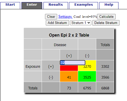
Figure 1. Data entry for 2X2 table at openepi.com.
Once the data are entered, click on the Calculate button to return a suite of results.
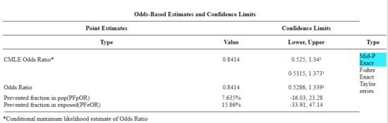
Figure 2. Results for 2X2 table at openepi.com.
Software: RcmdrPlugin.EBM
Note: Fall 2023 — I have not been able to run the EBM plugin successfully! Simply returns an error message — — on data sets which have in the past performed perfectly. Thus, until further notice, do not use the EBM plugin. Instead, use commands in the epiR package.
This isn’t the place nor can I be the author to discuss what evidence based medicine (EBM) entails (cf. Masic et al. 2008), or what its shortcomings may be (Djulbegovic and Guyatt 2017). Rcmdr has a nice plugin, based on the epiR package, that will calculate ARR, RRR and NNT as well as other statistics. The plugin is called RcmdrPlugin.EBM
install.packages("RcmdrPlugin.EBM", dependencies=TRUE)
After acquiring the package, proceed to install the plug-in. Restart Rcmdr, then select Tools and Rcmdr Plugins (Fig 3).
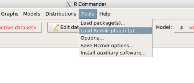
Figure 3. Rcmdr: Tools → Load Rcmdr plugins…
Find the EBM plug-in, then proceed to load the package (Fig 4).
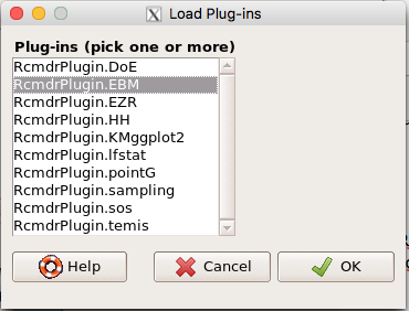
Figure 4. Rcmdr plug-ins available (after first download the files from an R mirror site).
Restart Rcmdr again and the menu “EBM” should be visible in the menu bar. We’re going to enter some data, so choose the Enter two-way table… option in the EBM plug-in (Fig 5)
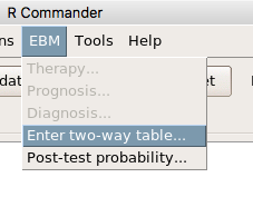
Figure 5. R Commander EBM plug-in, enter 2X2 table menus
To review, we have the following problem, illustrated with natural numbers and probability tree (Fig. 6).
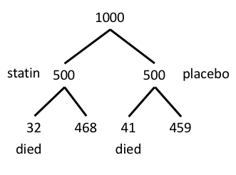
Figure 6. Illustration of probability tree for the statin problem
Now, let’s enter the data into the EBM plugin. For the data above I entered the counts as
| Lived | Died | |
| Statin | 468 | 32 |
| Placebo | 459 | 41 |
and selected the “Therapy” medical indicator (Fig 7)
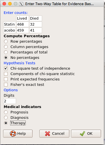
Figure 7. EBM plugin with two-way table completed for the statin problem.
The output from EBM plugin was as follows. I’ve added index numbers in brackets so that we can point to the output that is relevant for our worked example here.
(1) .Table <- matrix(c(468,32,459,41), 2, 2, byrow=TRUE, dimnames = list(c('Drug', 'Placebo'), c('Lived', 'Dead')))
(2) fncEBMCrossTab(.table=.Table, .x='', .y='', .ylab='', .xlab='', .percents='none', .chisq='1', .expected='0', .chisqComp='0', .fisher='0', .indicators='th', .decimals=2)
R output begins by repeating the commands used, here marked by lines (1) and (2). The statistics we want follow in the next several lines of output.
(3) Pearson's Chi-squared test data: .Table X-squared = 1.197, df = 1, p-value = 0.2739
(4) # Notations for calculations Event + Event -Treatment "a" "b" Control "c" "d"
(5)# Absolute risk reduction (ARR) = -1.8 (95% CI -5.02 - 1.42) %. Computed using formula: [c / (c + d)] - [a / (a + b)]
(6)# Relative risk = 1.02 (95% CI 0.98 - 1.06) %. Computed using formula: [c / (c + d)] / [a / (a + b)]
(7)# Odds ratio = 1.31 (95% CI 0.81 - 2.11). Computed using formula: (a / b) / (c / d)
(8) # Number needed to treat = -55.56 (95% CI 70.29 - Inf). Computed using formula: 1 / ARR
9)# Relative risk reduction = -1.96 (95% CI -5.57 - 1.53) %. Computed using formula: { [c / (c + d)] - [a / (a + b)] } / [c / (c + d)]
(10)# To find more about the results, and about how confidence intervals were computed, type \?epi.2by2 . The confidence limits for NNT were computed as 1/ARR confidence limits. The confidence limits for RRR were computed as 1 - RR confidence limits.
end R output
In summary, we found no difference between statin and placebo (P-value = 0.2739) and ARR of -1.8%
Questions
Data from a case-control study on alcohol use and esophageal cancer (Tuyns et al (1977), example from Gerstman 2014). Cases were men diagnosed with esophageal cancer from a region in France. Controls were selected at random from electoral lists from the same geographical region.
| Esophageal cancer | |||
|
Alcohol grams/day |
Cases | Noncases |
Total |
| > 80 | 96 | 109 |
205 |
|
< 80 |
104 |
666 |
770 |
| Total | 200 | 775 | 975 |
- What was the null hypothesis\? Be able to write the hypothesis in symbolic form and as a single sentence.
- What was the alternate hypothesis\? Be able to write the hypothesis in symbolic form and as a single sentence.
- What was the observed frequency of subjects with esophageal cancer in this study\? And the observed frequency of subjects without esophageal cancer\?
- Estimate Relative Risk, Absolute Risk, NNT, and Odds ratio\?
- Which is more appropriate, RR or OR\? Justify your decision.
- The American College of Obstetricians and Gynecologists recommends that women with an average risk of breast cancer (BC) over 40 get an annual mammogram. Nationally, the sensitivity of mammography is about 68% and specificity of mammography is about 75%. Moreover, mammography involves exposure of women to radiation, which is known to cause mutations. Given that the prevalence of BC in women between 40 and 49 is about 0.1%, please evaluate the value of this recommendation by completing your analysis.
A) In this age group, how many women are expected to develop BC\?
B) How many False negative would we expect\?
C) How many positive mammograms are likely to be true positives\? - “Less than 5% of women with screen-detectable cancers have their lives saved,” (quote from BMC Med Inform Decis Mak. 2009 Apr 2;9:18. doi: 10.1186/1472-6947-9-18): Using the information from question 5, What is the Number Needed to Treat for mammography screening\?
Chapter 7 contents
- Probability, Risk Analysis
- Epidemiology definitions
- Epidemiology basics
- Conditional Probability and Evidence Based Medicine
- Epidemiology: Relative risk and absolute risk, explained
- Odds ratio
- Confidence intervals
- References and suggested readings
7.3 – Conditional Probability and Evidence Based Medicine
- Introduction
- Probability and independent events
- Example of multiple, independent events
- Probabilistic risk analysis
- Conditional probability of non-independent events
- Diagnosis from testing
- Standard million
- Per capita rate
- Practice and introduce PPV and Youden’s J
- Evidence Based Medicine
- Software
- Example
- Questions
- Chapter 7 contents
Introduction
This section covers a lot of ground. We begin by addressing how probability of multiple events are calculated assuming each event is independent. The assumption of independence is then relaxed, and how to determine probability of an event happening given another event has already occurred, conditional probability, is introduced. Use of conditional probability to interpret results of a clinical test are also introduced, along with the concept of “evidence-based-medicine,” or EBM.
Probability and independent events
Probability distributions are mathematical descriptions of the probabilities of how often different possible outcomes occur. We also introduced basic concepts related to working with the probabilities involving more than one event.
For review, for independent events, you multiply the individual chance that each event occurs to get the overall probability.
Example of multiple, independent events

Figure 1. Now that’s a box full of kittens. Creative Commons License, source: https://www.flickr.com/photos/83014408@N00/160490011
What is the chance of five kittens in a litter of five to be of the same sex? In feral cat colonies, siblings in a litter share the same mother, but not necessarily the same father, superfecundation. Singleton births are independent events, thus the probability of the first kitten is female is 50%; the second kitten is female, also 50%; and so on. We can multiply the independent probabilities (hence, the multiplicative rule), to get our answer:
kittens <- c(0.5, 0.5, 0.5, 0.5, 0.5)
prod(kittens)
[1] 0.03125
Probabilistic risk analysis
Risk analysis is the use of information to identify hazards and to estimate the risk. A more serious example. Consider the 1986 Space Shuttle Challenger Disaster (Hastings 2003). Among the crew killed was Ellison Onizuka, the first Asian American to fly in space (Fig. 2, first on left back row). Onizuka was born and raised on Hawai`i and graduated from Konawaena High School in 1964.

Figure 2. STS-51-L crew: (front row) Michael J. Smith, Dick Scobee, Ronald McNair; (back row) Ellison Onizuka, Christa McAuliffe, Gregory Jarvis, Judith Resnik. Image by NASA – NASA Human Space Flight Gallery, Public Domain.
The shuttle was destroyed just 73 seconds after lift off (Fig. 3).

Figure 3. Space Shuttle Challenger launches from launchpad 39B Kennedy Space Center, FL, at the start of STS-51-L. Hundreds of shorebirds in flight. Image by NASA – NASA Human Space Flight Gallery, Public Domain.
This next section relies on material and analysis presented in the Rogers Commission Report June 1986. NASA had estimated that the probability of one engine failure would be 1 in 100 or 0.01; two engine failures would mean the shuttle would be lost. Thus, the probability of two rockets failing at the same time was calculated as 0.01 X 0.01, which is 0.0001 or 0.01%.
NASA had planned to fly the fleet of shuttles 100 times per year, which would translate to a shuttle failure once in 100 years. The Challenger launch on January 28, 1986, represented only the 25th flight of the shuttle fleet.
One difference on launch day was that the air temperature at Cape Canaveral was quite low for that time of year, as low as 22 °F overnight.
Attention was pointed at the large O-rings in the boosters (engines). In all, there were six of these O-rings. Testing suggested that, at the colder air temperatures, the chance that one of the rings would fail was 0.023. Thus, the chance of success was only 0.977. Assuming independence, what is the chance that the shuttle would experience O-ring failure?
shuttle <- c(0.977, 0.977, 0.977, 0.977, 0.977, 0.977)
#probability of success then was
prod(shuttle)
[1] 0.869

#and therefore probability of failure was
1 - prod(shuttle)
[1] 0.1303042
Conditional probability of non-independent events
But in many other cases, independence of events cannot be assumed. The probability of an event given that another event has occurred is referred to as conditional probability. Conditional probability is used extensively to convey risk. We’ve touched on some of these examples already:
- the risk of subsequent coronary events given high cholesterol;
- the risk of lung cancer given a person smokes tobacco;
- the risk of mortality from breast cancer given that regular mammography screening was conducted.
There are many, many examples in medicine, insurance, you name it. It is even an important concept that judges and lawyers need to be able to handle (e.g., Berry 2008).
A now famous example of conditional probability in the legal arena came from arguments over the chance that a husband or partner who beats his wife will subsequently murder her — this was an argument raised by the prosecution during pre-trial in the 1995 OJ Simpson trial (The People of the State of California v. Orenthal James Simpson), and successfully argued by O.J. Simpson’s attorneys… judge ruled in favor of the defense and evidence of OJ Simpson’s prior abuse were not included in trial). Gigerenzer (2002) and others have called this reverse Prosecutor’s Fallacy, where the more typical scenario is that the prosecution provides a list of probabilities about characteristics of the defendant, leaving the jury to conclude that no one else could have possibly fit the description.
In the OJ Simpson case, the argument went something like this. From the CDC we find that an estimated 1.3 million women are abused each year by their partner or former partner; each year about 1000 women are murdered. One thousand divided by 1.3 million is a small number, so even when there is abuse the argument goes, 99% of the time there is not murder. The Simpson judge ruled in favor of the defense and much of the evidence of abuse was excluded.
Something is missing from the defense’s argument. Nicole Simpson did not belong to a population of battered women — she belonged to the population of murdered women. When we ask, if a woman is murdered, what is the chance that she knew her murderer, we find that more than 55% knew their murderer — and of that 55%, 93% were killed by a current partner. The key is Nicole Simpson (and Ron Goldman) was murdered and OJ Simpson was an ex-partner who had been guilty of assault against Nicole Simpson. Now, it goes from an impossibly small chance, to a much greater chance. Conditional probability, and specifically Baye’s rule, is used for these kinds of problems.
Diagnosis from testing
Let’s turn our attention to medicine. A growing practice in medicine is to claim that decision making in medicine should be based on approaches that give us the best decisions. A search of PubMed texts for “evidence based medicine” found more than 91,944 (13 October 2021, and increase of thirteen thousand since last I looked (10 October, 2019). Evidence based medicine (EBM) is the “conscientious, explicit, judicious and reasonable use of modern, best evidence in making decisions about the care of individual patients” (Masic et al 2008). By evidence, we may mean results from quantitative, systematic reviews, meta-analysis, of research on a topic of medical interest, e.g., Cochrane Reviews.
Note 1: Primary research refers to generating or collecting original data in pursuit of tests of hypotheses. Both systematic reviews and meta-analysis are secondary research or “research on research.” As opposed to a literature review, systematic review make explicit how studies were searched for and included; if enough reasonably similar quantitative data are obtained through this process, the reviewer can combine the data and conduct an analysis to assess whether a treatment is effective (De Vries 2018).
As you know, no diagnostic test is 100% fool-proof. For many reasons, test results come back positive when the person truly does not have the condition — this is a false positive result. Correctly identifying individuals who do not have the condition, 100% – false positive rate, is called the specificity of a test. Think of specificity in this way — provide the test 100 true negative samples (e.g., 100 samples from people who do not have cancer) — how many times out of 100 does the test correctly return a “negative”? If 99 times out of 100, then the specificity rate for this test is 99%. Which is pretty good. But the test results mean more if the condition/disease is common; for rare conditions, even 99% is not good enough. Incorrect assignments are rare, we believe, in part because the tests are generally quite accurate. However, what we don’t consider is that detection and diagnosis from tests also depend on how frequent the incidence of the condition is in the population. Paradoxically, the lower the base rate, the poorer diagnostic value even a sensitive test may have.
To summarize our jargon for interpreting a test or assay, so far we have
- True positive (a), the person has a disease and the test correctly identifies the person as having the disease.
- False positive (b), test result incorrectly identifies disease; the person does not have the disease, but the test classifies the person as having the disease.
- False negative (c), test result incorrectly classifies person does not have disease, but the person actually has the disease.
- True negative (d), the person does not have the disease and the test correctly categorizes the person as not having the disease.
- Sensitivity of test is the proportion of persons who test positive and do have the disease (true positives):

If a test has 75% sensitivity, then out of 100 individuals who do have the disease, then 75 will test positive (TP = true positive). - Specificity of a test refers to the rate that a test correctly classifies a person that does not have the disease (TN = true negatives):

If a test has 90% specificity, then out of 100 individuals who truly do not have the disease, then 90 will test negative (= true negatives).
A worked example. A 50 year old male patient is in the doctor’s office. The doctor is reviewing results from a diagnostic test, e.g., a FOBT — fecal occult blood test — a test used as a screening tool for colorectal cancer (CRC). The doctor knows that the test has a sensitivity of about 75% and specificity of about 90%. Prevalence of CRC in this age group is about 0.2%. Figure 4 shows our probability tree using our natural numbers approach (Fig. 4).
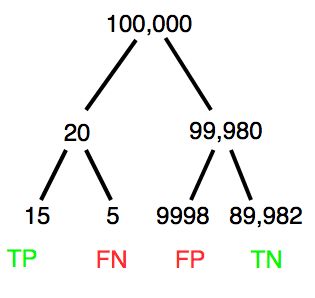
Figure 4. Probability tree for FOBT test; Good test outcomes shown in green: TP stands for true positive and TN stands for true negative. Poor outcomes of a test shown in red: FN stands for false negative and FP stands for false positive.
The associated probabilities for the four possible outcomes of these kinds of tests (e.g., what’s the probability of a person who has tested positive in screening tests actually has the disease?) are shown in Table 1.
Table 1. A 2 X 2 table of possible outcomes of a diagnostic test.
| Person really has the disease | ||
| Test Result | Yes | No |
| Positive | a TP |
b FP |
| Negative | c FN |
d TN |
Baye’s rule is often given in probabilities,
![\begin{align*} p\left ( D\mid \oplus \right )=\frac{p\left ( D \right )\cdot p\left (\oplus\mid D \right )}{[p\left ( D \right )\cdot p\left (\oplus \right )+p\left ( ND \right )\cdot p\left (\oplus \mid ND \right )]} \end{align*}](https://biostatistics.letgen.org/wp-content/ql-cache/quicklatex.com-fd988801ed9f7a29c963f2df79fcf35c_l3.png "Rendered by QuickLaTeX.com")
Baye’s rule, where truth is represented by either D (the person really does have the disease”) or ND (the person really does not have the disease”) and ⊕ is symbol for “exclusive or” and reads “not D” in this example.
An easier way to see this is to use frequencies instead. Now, the formula is

Simplified Baye’s rule, where a is the number of people who test positive and DO HAVE the disease and b is the number of people who test positive and DO NOT have the disease.
Standardized million
Where did the 100,000 come from? We discussed this in chapter 2: it’s a simple trick to adjust rates to the same population size. We use this to work with natural numbers instead of percent or frequencies. You choose to correct to a standardized population based on the raw incidence rate. A rough rule of thumb:
Table 2. Relationship between standard population size and incidence rate.
| Raw IR rate about | IR | Standard population |
| 1/10 | 10% | 1000 |
| 1/100 | 1% | 10,000 |
| 1/1000 | 0.1% | 100,000 |
| 1/10,000 | 0.01% | 1,000,000 |
| 1/100,000 | 0.001% | 10,000,000 |
| 1/1,000,000 | 0.0001% | 100,000,000 |
The raw incident rate is simply the number of new cases divided by the total population.
Per capita rate
Yet another standard manipulation is to consider the average incidence per person, or per capita rate. The Latin “per capita” translates to “by head” (Google translate), but in economics, epidemiology, and other fields it is used to reflect rates per person. Tuberculosis is a serious infectious disease of primarily the lungs. Incidence rates of tuberculosis in the United States have trended down since the mid 1900s: 52.6 per 100K in 1953 to 2.7 per 100K in 2019 (CDC). Corresponding per capita values are 5.26 x 10⁻⁴ and 2.7 x 10⁻⁵, respectively. Divide the rate by 100,000 to get per person rate.
Practice and introduce PPV and Youden’s J
Let’s break these problems down, and in doing so, introduce some terminology common to the field of “risk analysis” as it pertains to biology and epidemiology. Our first example considers the fecal occult blood test, FOBT, test. Blood in the stool may (or may not) indicate polys or colon cancer. (Park et al 2010).
The table shown above will appear again and again throughout the course, but in different forms.
Table 3. A 2 X 2 table of possible outcomes of FOBT test.
| Person really has the disease | |||
| Yes | No | ||
| Positive | 15 | 9998 | PPV = 15/(15+9998) = 0.15% |
| Negative | 5 | 89,982 | NPV = 89982/(89982+5) = 99.99% |
We want to know how good is the test, particularly if the goal is early detection? This is conveyed by the PPV, positive predictive value of the test. Unfortunately, the prevalence of a condition is also at play: the lower the prevalence, the lower the PPV must be, because most positive tests will be false when population prevalence is low.
Youden (1950) proposed a now widely adopted index that summarizes how effective a test is. Youden’s J is the sum of specificity and sensitivity minus one.

where Se stands for sensitivity of the test and Sp stands for sensitivity of the test.
Youden’s J takes on values between 0, for a terrible test, and 1, for a perfect test. For our FOBT example, Youden’s J was 0.65. This statistic looks like it’s independent of prevalence, but it’s use as a decision criterion (e.g., a cutoff value, above which test is positive, below test is considered negative), assumes that the cost of misclassification (false positives, false negatives) are equal. Prevalence affects number of false positives and false negatives for a given diagnostic test, so any decision criterion based on Youden’s J will also be influenced by prevalence (Smits 2010).
Another worked example. A study on cholesterol-lowering drugs (statins) reported a relative risk reduction of death from cardiac event by 22%. This does not mean that for every 1000 people fitting the population studied, 220 people would be spared from having a heart attack. In the study, the death rate per 1000 people was 32 for the statin versus 41 for the placebo — recall that a placebo is a control treatment offered to overcome potential patient psychological bias (see Chapter 5.4). The absolute risk reduction due to statin is only 41 – 32 or 9 in 1000 or 0.9%. By contrast, relative risk reduction is calculated as the ratio of the absolute risk reduction (9) divided by the proportion of patients who died without treatment (41), which is 22% (LIPID Study Group 1998).
Note that risk reduction is often conveyed as a relative rather than as an absolute number. The distinction is important for understanding arguments based in conditional probability. Thus, the question we want to ask about a test is summarized by absolute risk reduction (ARR) and number needed to treat (NNT), and for problems that include control subjects, relative risk reduction (RRR). We expand on these topics in the next section, 7.4 – Epidemiology: Relative risk and absolute risk, explained.
Evidence Based Medicine
One culture change in medicine is the explicit intent to make decisions based on evidence (Masic et al 2008). Of course, the joke then is, well, what were doctors doing before, diagnosing without evidence? The comic strip xkcd offers one possible answer (Fig. 5).
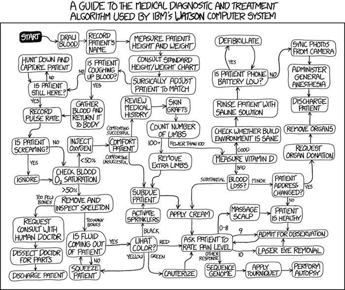
Figure 5. A summary of “evidence based medical” decisions, perhaps? https://xkcd.com/1619/
As you can imagine, there’s considerable reflection about the EBM movement (see discussions in response to Accad and Francis 2018, e.g., Goh 2018). More practically, our objective is for you to be able to work your way through word problems involving risk analysis. You can expect to be asked to calculate, or at least set up for calculation, any of the statistics listed above (e.g., False negative, false positive, etc.). Practice problems are listed at the end of this section, and additional problems are provided to you (Homework 4). You’ll also want to check your work, and in any real analysis, you’d most likely want to use R.
Software
R has several epidemiology packages, and with some effort, can save you time. Another option is to run your problems in OpenEpi, a browser-based set of tools. OpenEpi is discussed with examples in the next section, 7.4.
Here, we illustrate some capabilities of the epiR package, expanded more also in the next section, 7.4. We’ll use the example from Table 3.
R code
library(epiR)
Table3 <- matrix(c(15, 5, 9998, 89982), nrow = 2, ncol = 2)
epi.tests(Table3)
R output
         Outcome + Outcome -   Total
Test +          15      9998   10013
Test -           5     89982   89987
Total           20     99980  100000

Point estimates and 95% CIs:
--------------------------------------------------------------
Apparent prevalence *                      0.10 (0.10, 0.10)
True prevalence *                          0.00 (0.00, 0.00)
Sensitivity *                              0.75 (0.51, 0.91)
Specificity *                              0.90 (0.90, 0.90)
Positive predictive value *                0.00 (0.00, 0.00)
Negative predictive value *                1.00 (1.00, 1.00)
Positive likelihood ratio                  7.50 (5.82, 9.67)
Negative likelihood ratio                  0.28 (0.13, 0.59)
False T+ proportion for true D- *          0.10 (0.10, 0.10)
False T- proportion for true D+ *          0.25 (0.09, 0.49)
False T+ proportion for T+ *               1.00 (1.00, 1.00)
False T- proportion for T- *               0.00 (0.00, 0.00)
Correctly classified proportion *          0.90 (0.90, 0.90)
--------------------------------------------------------------
* Exact CIs
Oops! I wanted PPV, which by hand calculation was 0.15%, but R reported “0.00?” This is a significant figure reporting issue. The simplest solution is to submit options(digits=6) before the command, then save the output from epi.tests() to an object and use summary(). For example
options(digits=6)
myEpi <- epi.tests(Table3)
summary(myEpi)
And R returns
     statistic           est        lower        upper
1           ap  0.1001300000 0.0982761568  0.102007072
2           tp  0.0002000000 0.0001221693  0.000308867
3           se  0.7500000000 0.5089541283  0.913428531
4           sp  0.9000000000 0.8981238085  0.901852950
5      diag.ac  0.8999700000 0.8980937508  0.901823014
6      diag.or 27.0000000000 9.8110071871 74.304297826
7         nndx  1.5384615385 1.2265702376  2.456532054
8       youden  0.6500000000 0.4070779368  0.815281481
9       pv.pos  0.0014980525 0.0008386834  0.002469608
10      pv.neg  0.9999444364 0.9998703379  0.999981958
11      lr.pos  7.5000000000 5.8193604069  9.666010707
12      lr.neg  0.2777777778 0.1300251423  0.593427490
13      p.rout  0.8998700000 0.8979929278  0.901723843
14       p.rin  0.1001300000 0.0982761568  0.102007072
15      p.tpdn  0.1000000000 0.0981470498  0.101876192
16      p.tndp  0.2500000000 0.0865714691  0.491045872
17      p.dntp  0.9985019475 0.9975303919  0.999161317
18      p.dptn  0.0000555636 0.0000180416  0.000129662
There we go — pv.pos reported as 0.0014980525, which, after turning to a percent and rounding, we have 0.15%. Note also the additional statistics provided — a good rule of thumb — always try to save the output to an object, then view the object, e.g., with summary(). Refer to help pages for additional details of the output (?epi.tests).
What about R Commander menus?
Note 2: Fall 2023 — I have not been able to run the EBM plugin successfully! Simply returns an error message — — on data sets which have in the past performed perfectly. Thus, until further notice, do not use the EBM plugin. Instead, use commands in the epiR package. I’m leaving the text here on the chance the error with the plugin is fixed.
Rcmdr has a plugin that will calculate ARR, RRR and NNT. The plugin is called RcmdrPlugin.EBM (Leucuta et al 2014) and it would be downloaded as for any other package via R.
Download the package from your selected R mirror site, then start R Commander.
install.packages("RcmdrPlugin.EBM")
From within R Commander (Fig. 6), select
Tools → Load Rcmdr plug-in(s)…
Figure 6. To install an Rcmdr plugin, first go to Rcmdr → Tools → Load Rcmdr plug-in(s)…
Next, select from the list the plug-in you want to load into memory, in this case, RcmdrPlugin.EBM (Fig 7).
Figure 7. Select the Rcmdr plugin, then click the “OK” button to proceed.
Restart Rcmdr again (Fig. 8),
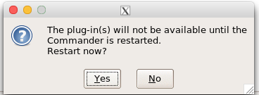
Figure 8. Select “Yes” to restart R Commander and finish installation of the plug-in.
and the menu “EBM” should be visible in the menu bar (Fig. 9).
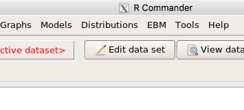
Figure 9. After restart of R Commander the EBM plug-in is now visible in the menu.
Note that you will need to repeat these steps each time you wish to work with a plug-in, unless you modify your .RProfile file. See
Rcmdr → Tools → Save Rcmdr options…
Clicking on the EBM menu item brings up the template for the Evidence Based Medicine module. We’ll mostly work with 2 X 2 tables (e.g., see Table 1) , so select the “Enter two-way table…” option to proceed (Fig. 10).
Figure 10. Select “Enter two-way table…”.
And finally, Figure 11 shows the two-way table entry cells along with options. We’ll try a problem by hand then use the EBM plugin to confirm and gain additional insight.
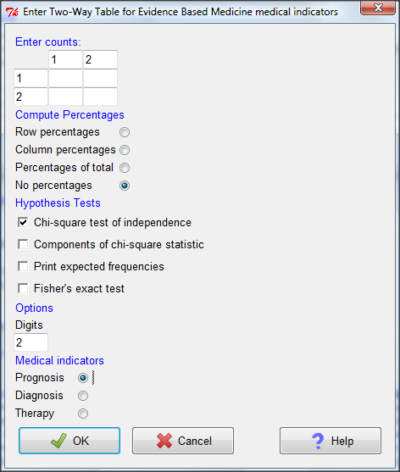
Figure 11. Two-way table Rcmdr EBM plug-in.
For assessing how good a test or assay is, use the Diagnosis option in the EBM plugin. For situations with treated and control groups, use Therapy option. For situations in which you are comparing exposure groups (e.g., smokers vs non-smokers), use the Prognosis option.
Example
Here’s a simple one (problem from Gigerenzer 2002).
About 0.01% of men in Germany with no known risk factors are currently infected with HIV. If a man from this population actually has the disease, there is a 99.9% chance the tests will be positive. If a man from this population is not infected, there is a 99.9% chance that the test will be negative. What is the chance that a man who tests positive actually has the disease?
Start with the reference, or base population (Figure 12). It’s easy to determine the rate of HIV infection in the population if you use numbers. For 10,000 men in this group, exactly one man is likely to have HIV (0.0001X10,000), whereas 9,999 would not be infected.
For the man who has the disease it’s virtually certain that his results will be positive for the virus (because the sensitivity rate = 99.9%). For the other 9,999 men, one will test positive (the false positive rate = 1 – specificity rate = 0.01%).
Thus, for this population of men, for every two who test positive, one has the disease and one does not, so the probability even given a positive test is only 100*1/2 = 50%. This would also be the test’s Positive Predictive Value.
Note that if the base rate changes, then the final answer changes! For example, if the base rate was 10%
It also helps to draw a tree to help you determine the numbers (Fig. 12)
Figure 12. Draw a probability tree to help with the frequencies.
From our probability tree in Figure 12 it is straight-forward to collect the information we need.
- Given this population, how many are expected to have HIV? Two.
- Given the specificity and sensitivity of the assay for HIV, how many persons from this population will test positive? Two.
- For every positive test result, how many men from this population will actually have HIV? One.
Thus, given this population with the known risk associated, the probability that a man testing positive actually has HIV is 50% (=1/(1+1)).
Use the EBM plugin. Select two-way table, then enter the values as shown in Fig. 13.
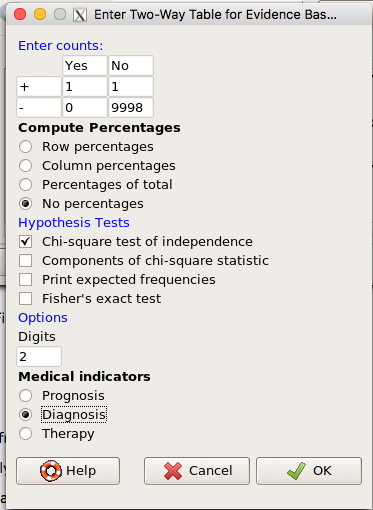
Figure 13. EBM plugin with data entry
Select the “Diagnosis” option — we are answering the question: How probable is a positive result given information about sensitivity and specificity of a diagnosis test. The results from the EBM functions are given below
Rcmdr> .Table
      Yes No
   +  1    1
   -  0 9998
Rcmdr> fncEBMCrossTab(.table=.Table, .x='', .y='', .ylab='', .xlab='',
Rcmdr+ .percents='none', .chisq='1', .expected='0', .chisqComp='0', .fisher='0',
Rcmdr+ .indicators='dg', .decimals=2)
# Notations for calculations
        Disease + Disease -
Test +      "a"         "b"
Test -      "c"         "d"
# Sensitivity (Se) = 100 (95% CI 2.5 - 100) %. Computed using formula: a / (a + c)
# Specificity (Sp) = 99.99 (95% CI 99.94 - 100) %. Computed using formula: d / (b + d)
# Diagnostic accuracy (% of all correct results) = 99.99 (95% CI 99.94 - 100) %. Computed using formula: (a + d) / (a + b + c + d)
# Youden's index = 1 (95% CI 0.02 - 1). Computed using formula: Se + Sp - 1
# Likelihood ratio of a positive test = 9999 (95% CI 1408.63 - 70976.66). Computed using formula: Se / (Sp - 1)
# Likelihood ratio of a negative test = 0 (95% CI 0 - NaN). Computed using formula: (1 - Se) / Sp
# Positive predictive value = 50 (95% CI 1.26 - 98.74) %. Computed using formula: a / (a + b)
# Negative predictive value = 100 (95% CI 99.96 - 100) %. Computed using formula: d / (c + d)
# Number needed to diagnose = 1 (95% CI 1 - 40.91). Computed using formula: 1 / [Se - (1 - Sp)]
Note that the formula’s used to calculate Sensitivity, Specificity, etc., follow our Table 1 (compare to “Notations for calculations”). The use of EBM provides calculations of our confidence intervals.
Questions
- The sensitivity of the fecal occult blood test (FOBT) is reported to be 0.68. What is the False Negative Rate?
- The specificity of the fecal occult blood test (FOBT) is reported to be 0.98. What is the False Positive Rate?
- For men between 50 and 54 years of age, the rate of colon cancer is 61 per 100,000. If the false negative rate of the fecal occult blood test (FOBT) is 10%, how many persons who have colon cancer will test negative?
- For men between 50 and 54 years of age, the rate of colon cancer is 61 per 100,000. If the false positive rate of the fecal occult blood test (FOBT) is 10%, how many persons who do not have colon cancer will test positive?
- A study was conducted to see if mammograms reduced mortality
Mammogram Deaths/1000 women No 4 Yes 3 data from Table 5-1 p. 60 Gigerenzer (2002)
What is the RRR? - A study was conducted to see if mammograms reduced mortality
Mammogram Deaths/1000 women No 4 Yes 3 data from Table 5-1 p. 60 Gigerenzer (2002)
What is the NNT? - Does supplemental Vitamin C decrease risk of stroke in Type II diabetic women? A study conducted on 1923 women, a total of 57 women had a stroke, 14 in the normal Vitamin C level and 32 in the high Vitamin C level. What is the NNT between normal and high supplemental Vitamin C groups?
- Sensitivity of a test is defined as
A. False Positive Rate
B. True Positive Rate
C. False Negative Rate
D. True Negative Rate - Specificity of a test is defined as
A. False Positive Rate
B. True Positive Rate
C. False Negative Rate
D. True Negative Rate - In thinking about the results of a test of a null hypothesis, Type I error rate is equivalent to
A. False Positive Rate
B. True Positive Rate
C. False Negative Rate
D. True Negative Rate - During the Covid-19 pandemic, number of reported cases each day were published. For example, 155 cases were reported for 9 October 2020 by Department of Health. What is the raw incident rate?
Chapter 7 contents
- Introduction
- Epidemiology definitions
- Epidemiology basics
- Conditional Probability and Evidence Based Medicine
- Epidemiology: Relative risk and absolute risk, explained
- Odds ratio
- Confidence intervals
- References and suggested readings
1.1 – A quick look at R and R Commander
A first look at R
.
R is a programming language for statistical computing (Venables et al 2009). R is an interpreted language — when you run (execute) an R program — the R interpreter intercepts and runs the code immediately through its command-line interface, one line at time. Python is another popular interpreted language common in data science. Interpreted languages are in contrast to compiled languages, like C++ and Rust, where program code is sent to a compiler to a machine language application.
The following steps user through use of R and R Commander, from installation to writing and running commands. Mike’s Workbook for Biostatistics has a ten-part tutorial, A quick look at R and R Commander, which I recommend.
Note: Getting started? By all means rely on Mike’s Biostatistics Book and blogs or other online tutorials to point you in the right direction. You’ll also find many free and online books that may provide the right voice to get you working with R. However, the best way to learn is to go to the source. The R team has provided extensive documentation, all included as part of your installation of R. In R, run the command RShowDoc("doc name"). replace doc name with the name of the R manual or R user guide. For example, the Venables publication is accessed as RShowDoc("R-intro"). Similarly, the manual for installation is RShowDoc("R-admin") and the manual for R data import/export is RShowDoc("R-data").
Install R
.
Full installation instructions are available at Install R, and for the R Commander package, at Install R Commander. Here, we provide a brief overview of the installation process.
Note: The instructions at Mike’s Biostatistics Book assume use of R on a personal computer running updated Microsoft Windows or Apple macOS operating systems. For Linux instructions, e.g., Ubuntu distro, see How to install R on Ubuntu 22.04. For Chromebook users, if you can install a Linux subsystem, then you can also install and run R although it’s not a trivial installation. For instructions to install R see Levi’s excellent writeup at levente.littvay.hu/chromebook/. (This works best with Intel-based CPUs — see my initial attempts with an inexpensive Chromebook at Install R.)
Another option is to run R in the cloud via service like Google’s Colab or CoCalc hosted by SageMath. Both support Jupyter Notebooks, a “web-based interactive computational environment.” Neither cloud-based service supports use of R Commander (because R Commander interacts with your local hardware). Colab is the route I’d choose if I don’t have access to a local installation of R. See Use R in the cloud for more details.
Download a copy of the R installation file appropriate for your computer from one of the Comprehensive R Archive Network (CRAN) mirror site of the r-project.org. For Hawaii, the most convenient mirror site is provided by the folks at RStudio (https://cloud.r-project.org/.
In brief, Windows 11 users download and install the base distribution. MacOS users must first download and install XQuartz (https://Xquartz.org), which provides the X Window System needed by R’s GUI (graphic user interface). Once XQuartz is installed, proceed to install R to your computer. MacOS users — don’t forget to drag the R.app to your Applications folder!
Start R
.
The following is a minimal look at how to use R and R Commander. Please refer to tutorials at Mike’s Workbook for Biostatistics (R work, part 1 – 10) to learn use of R and R Commander.
We’re just getting started, so the next thing to learn is how to set your working environment for your R sessions. Although we’ll discuss the R environment more as we proceed, it’s a good idea to start with a best practice action common in data science — always create and work from a working folder. This can be a local folder on your computer or pointed to a folder in your cloud storage. On my mac I usually create a folder on the desktop, example BI311, and point to that as my working folder for a project. Now, we need to point R to use the working folder — we do this at start of each R session (or modify some code R needs during start up to always point to the folder — for now, we leave that for a later exercise).
Once R is installed on your computer, start R as you would any program on your computer. For example, the icon for the R.app as it appears in the dock on a MacBook is shown in Figure 1.

Figure 1. R.app icon shown on a MacBook dock.
To point R to our working folder, there are several options. For now, we’ll go with writing and submitting a simple function in R. Recall that R has a command-line. The R prompt appears on the command line in the RGUI as the greater-than typographical symbol “>” at the beginning of a line (Fig 2). The prompt is returned by R to indicate the interpreter is ready to accept the next line of code.
First, discover where R is pointing to by submitting (type the command exactly as written then select the enter/return key) the function getwd() at the prompt. On my macbook, R returns
> getwd()
[1] "/Users/[username]/Documents"
To point to my working folder, I submit setwd("/Users/[username]/Desktop/BI311". When I run getwd() again, R returns the update
> getwd()
[1] "/Users/[username]/Desktop/BI311"
Note: Windows users will recognize that, unlike macOS and Linux, they will need to write paths with the backslash, not the forward slash. This is discussed further in Mike’s Workbook.
[username] is just a place holder here — no reason to share my actual user name!
Ready to do some work?
Where discussion requires reference to instructions on use of the R programming language, R code (instructions) the user needs to enter at the R prompt are shown in code blocks.
Courier New font within a “code block.”Until you write your own functions, the general idea is, you enter one set of commands at a time, one line at a time. For example, to create a new variable, curry.points, containing points scored by the NBA’s Steph Curry during the 2016 playoffs, type the following code at the R prompt (displayed as >, the “greater than” sign)
curry.points <- c(24,6,40,29,26,28,24,19,31,31,11,18,19).
and to obtain the mean, or arithmetic average, for curry.points at the R prompt type and enter
.
mean(curry.points).
Output from R function mean will look like the following
.
[1] 24.42857.
The R prompt appears in the RGUI as the greater-than typographical symbol “>” at the beginning of a line (Fig 2). The prompt is returned by R to indicate the interpreter is ready to accept the next line of code.

Figure 2. The R GUI on a macOS system; red arrow points to the R prompt.
Everything that exists is an object
.
A brief programmer’s note — John M. Chambers, creator of the S programming language and a member of the R-project team, once wrote that sub-header phrase about R and objects. What that means for us: programming objects can be a combination of variables, functions, and data structures. During an R session the user creates and uses objects. The ls() function is a useful R command to list objects in memory. If you have been following along with your own installed R app, then how many objects are currently available in your session of R? Answer by submitting ls(). Hint: the answer should be one object.
A routine task during analysis is to calculate an estimate then use the result in subsequent work. For example, instead of simply printing the result of mean(curry.points), we can assign the result to an object.
myResult <- mean(curry.points)
.
To confirm the new object was created, try ls() again. And, of course, there’s no particular reason to use the object name, myResult, I provided! Like any programming language, creating good object names will make your code easier to understand.
When you submit the above code, R returns the prompt, and the result of the function call is not displayed. View the result by submitting the object’s name at the R prompt, in this case, myResult. Alternatively, a simple trick is to string commands on the same line by adding ; (semicolon) at the end of the first command. For example,
myResult <- mean(curry.points); myResult
.
Write your code as script
.
While it is possible to submit code one line at a time, a much better approach is to create and manage code in a script file. A script file is just a text file with one command per line, but potentially containing many lines of code. Script files help automate R sessions. Once the code is ready, the user submits code to R from the script file.
Note: Working with scripts eliminates the R prompt, but code is still interpreted one line at a time. The user does not type the prompt in a script file.
Figure 3 shows how to create a new script file via the RGUI menu: File → New script.

Figure 3. Screenshot of drop down menu RGUI, create new script, Windows 10.
The default text editor opens (Fig 4).

Figure 4. Screenshot of portion of R Script editor, Windows 11. A simple R command is visible.
Submit code by placing cursor at start of the code or, if code consists of multiple lines, select all of the code, then hit keyboard keys Ctrl+R (Windows 11) or for macOS, Cmd+Enter.
By default, save R script files for reuse with the file extension .R, e.g., myScript.R. Because the scripts are just text files you can use other editors that may make coding more enjoyable (see RStudio in particular, but there are many alternatives, some free to use. A good alternative is ESS).
Install R Commander package
.
By now, you have installed the base package of the R statistical programming language. The base package contains all of the components you would need to create and run data analysis and statistics on sets of data. However, you would quickly run into the need to develop functions, to write your own programs to facilitate your work. One of the great things about R is that a large community of programmers have written and contributed their own code; chances are high that someone has already written a function you would need. These functions are submitted in the form of packages. Throughout the semester we will install several R packages to extend R capabilities. R packages discussed in this book are listed at R packages of the Appendix.
Our first package to install is R Commander, Rcmdr for short. R Commander is a package that adds function to R; it provides a familiar point-and-click interface to R, which allows the user to access functions via a drop-down menu system (Fox 2017). Thus, instead of writing code to run a statistical test, Rcmdr provides a simple menu driven approach to help students select and apply the correct statistical test. R Commander also provides access to Rmarkdown and a menu approach to rendering reports.
install.packages("Rcmdr")
.
In addition, download and install the plugin
install.packages("RcmdrMisc")
See Install R Commander for detailed installation instructions.
Plugins are additional software which add function to an existing application.
Start R Commander
.
After installing Rcmdr, to start R Commander, type library(Rcmdr) at the R prompt and enter to load the library
library(Rcmdr).
On first run of R Commander you may see instructions for installing additional packages needed by R Commander. Accept the defaults and proceed to complete the installation of R Commander. Next time you start R commander the start up will be much faster since the additional packages needed by R Commander will already be present on your computer.
Note that you don’t type the R prompt and, indeed, in R Commander Script window you won’t see the prompt (Fig 4). Instead, you enter code in the R Script window, then click “Submit” button (or Win11: Ctrl+R or for macOS: Cmd+Enter), to send the command to the R interpreter. Results are sent to Output window (Fig 5).
 Rcmdr ver. 2.4-4.")
Figure 5. The windows of R Commander, macOS. From bottom to top: Messages, Output, Script (tab, Markdown) Rcmdr ver. 2.4-4.
Figure 5 shows how the R Commander GUI looks on a macOS computer. The look is similar on Microsoft Windows 11 machines (Fig 6).
 Rcmdr ver. 2.5-1.")
Figure 6. The windows of R Commander, Win11. From bottom to top: Messages, Output, Script (tab, R Markdown) Rcmdr ver. 2.5-1.
We use R Commander because it gives us access to code from drop-down menus, which at least initially, helps learn R (Fox 2005, Fox 2016). Later, you’ll want to write the code your self, and RStudio provides a nice environment to accomplish your data analysis.
Improve Rcmdr experience
Windows users: R Commander works best in Windows if SDI option is set. This can be accomplished during R installation (“Startup options” popup, change from default “No” to “Yes” to customize), but you can also change after installing R. Win11 users should change from MDI to SDI — from one big window to separate windows — (see Do explore settings, Figure 5). The downside of SDI is that while multiple Windows may appear during an R session, one or more windows may be hidden by an open window. For example, plots will popup in a new window and may be obscured by the Rcmdr window if full screen. A simple trick to view active windows on Win11 is to use the keyboard shortcut Alt+Tab to view and cycle between windows. What about SDI and RStudio? RStudio experience will be similar whether MDI (default) or SDI was selected.
macOS users: To improve R Commander performance, turn off Apple’s app nap (see Do explore settings, Figures 6 & 7), which should improve a Mac user’s experience with R Commander and other X Window applications.
Complete R setup by installing LaTeX and pandoc for Markdown
.
LaTeX is a system for document preparation. pandoc is a document converter system. Markdown is a language used to create formatted writing from simple text code. Once these supporting apps are installed, sophisticated reports can be generated from R sessions, by-passing copy and paste methods one might employ. See Install R Commander for instructions to add these apps.
Note: If you successfully installed R and are running R Commander, but may be having problems installing pandoc or LaTeX, then this note is for you. While there’s advantages to getting pandoc etc working, it is not essential for BI311 work.
Assuming you have Rcmdr and RcmdrMisc installed, and if you have started Rcmdr and have it up and running, then we can skip pandoc and LaTeX installation and use features of your browser to save to pdf.
R Markdown by default will print to a web page (an html document called RcmdrMarkdown.html) and display it in your default browser. To meet requirements of BI311 — you submit pdf files — we can print the html document generated from “Generate Report” in R Commander to a pdf.
- Chrome browser, right click in the web page, from the popup menu select Print, then change destination to Save as pdf.
- Safari browser, right click then select Print page (or if an option, Save page as pdf), then find at lower left find PDF and option to Save as PDF.
R Markdown
.
Markdown is a syntax for plain text formatting and is really helpful for generating clean html (web) files. R Commander also helps us with our reporting. R Markdown is provided as a tab (Fig 4, 5). Provided you have also installed pandoc on your computer, you can also convert or “render” the work into other formats including pdf and epub. Unsure if your computer has pandoc installed? If you are unsure than most likely it is not installed. 😁 Rcmdr provides a quick check — go to Tools and if you see Install auxiliary software, then click on it and a link to pandoc website to find and download installation file. You can also confirm install of pandoc by opening a terminal on your computer (e.g., search “terminal” on macOS or “cmd” on Win11), then enter pandoc –version at the shell prompt. Figure 7 shows version pandoc is installed on my Win11 HP laptop.
 on win11 computer, checking for installed pandoc on a win10 pc.")
Figure 7. Screenshot of terminal window (cmd) on win11 computer, checking for installed pandoc on a win10 pc.
Enter your R code in the script window, submit your code, and your results (code, output, graphs) are neatly formatted for you by Markdown. Once the Markdown file is created in R Commander, you can then export to an html file for a a web browser, an MS Word document, or other modes.
Do explore settings!
.
After installation, R and R Commander are ready to go. However, students are advised that a few settings may need to be changed to improve performance. For example, on Win11 PCs, R Commander recommends changing from the default MDI (Multiple Document Interface) to SDI (Single Document Interface). Check the SDI button via Edit menu, select GUI preferences menu. Click save, which will make changes to .RProfile, then exit and restart R. Check to make sure the changes have been made (Fig 8).

Figure 8. Screenshot of GUI preferences settings after changing from default MDI to SDI, win10
For macOS users, both R and Rcmdr will run better if you turn off Apple’s power saving feature called nap. From Rcmdr go to Tools and select Manage Mac OS X app nap for R.app… (Fig 9).

Figure 9. Screenshot Rcmdr Tools popup menu, macOS 10.15.6
A dialog box appears; select off to turn off app nap (Fig 10).

Figure 10. Screenshot Rcmdr Set app nap dialog box, macOS 10.15.6
Exit R Commander
.
Click on Rcmdr: File → Exit, then choose to exit from just R Commander, or both R Commander and R.
If you exit just R Commander or both R and R Commander, you’ll receive a pop-up request to confirm you want to quit R Commander (click yes), and a second prompt asking if you want to save your script. In general, select yes and then you’ll be able to take up where you left off. Similarly, if asked to save your workspace, choose no. If you save workspace, this creates an .RProfile text file with settings for how R and R Commander will behave the next time you start R. The file will be saved to your current working folder, which R will use the next time R starts. At least while you are getting started, you should avoid creating these .RProfile files.
As long as the current session of R is active, then the library for Rcmdr, as well as any other library loaded during the R session, is in memory. To start R Commander again while R is running, at the R prompt, type and submit
Commander()
.
Questions
.
- Biostatistics students should work through my ten R lessons, A quick look t R and R Commander, available in Mike’s Workbook for Biostatistics.
- Students should also search Internet for R tutorials and R Commander tutorials. Find recent tutorials and work through several of them. We get better when we practice.
Quiz
Chapter 1 contents
.
- Getting started
- A quick look at R and R Commander
- Chapter 1 – References