12.6 – ANOVA posthoc tests

Introduction
Performing multiple comparisons and the one-way ANOVA
Questions
Data set
Chapter 12 contents

Introduction

Tests of the null hypothesis in a one-way ANOVA yields one answer: either you reject the null, or you do not reject the null hypothesis — with the usual caveats about “provisionally reject,” etc (Ch8.2 and Ch8.3). But while there was only one factor (population, drug treatment, etc) in a one-way ANOVA, there are usually many treatments (e.g., multiple levels, four different populations, three doses of a drug plus a placebo).

ANOVA plus posthoc tests solves the multiple comparison problem we discussed: you still get your tests of all group differences, but with adjustments to the procedures so that these tests are conducted without suffering the increase in Type I error = the multiple comparison problem. If the null hypothesis is rejected, you may then proceed to posthoc tests among the groups to identify differences.

Consider the following example of four populations scored for some outcome, sim.ch12 (scroll down the page, or click here to get the R code).

Bring the data frame, sim.ch12, into current memory in Rcmdr by selecting the data set. Next, run the one-way ANOVA.

Rcmdr: Statistics → Means → One-way ANOVA…

which brings up the following menu (Fig. 1)

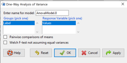
Figure 1. One-way ANOVA menu in R Commander

Figure 1. One-way ANOVA menu in R Commander

Note: If you look carefully in Figure 1, you can see model name was AnovaModel.8. There’s nothing significant about that name, it just means this was the 8^th model I had run up to that point. As a reminder, Rcmdr will provide names for models for you; it is better practice to provide model names yourself.

Notice that Rcmdr menu correctly identifies the Factor variable, which contains text labels for each group, and the Response variable, which contains the numerical observations.

Note: If your factor is numeric, you’ll first have to tell R that the variable is a factor and hence nominal. this can be accomplished within Rcmdr via the Data → Manage variables… options, or simply submit the command

newName <- as.factor(oldVariable)

If your data set contains more variables, then you would need to sort through these and select the correct model (Fig. 1).

To get the default Tukey posthoc tests simply check the Pairwise comparisons box and then click OK.

For a test of the null that four groups have the same mean, a publishable ANOVA table would look like Table 1.

Note: the ANOVA table is something you put together from the output of R (or other statistical programs). After running one-way ANOVA in Rcmdr, go to Models → Hypothesis tests → ANOVA table…, accept the defaults (marginality, sandwich estimators and are explained in the next chapter 12.7).

Table 1. The ANOVA table

	Df	Mean Square	F	P†
Label	3	389627	76.44	< 0.0001
Error	36	61167

† DrD edited the R output for one-tailed p-value from 1.108357e-15 to a threshold < 0.0001.

Note: To automatically replace a small p-value with a threshold cutoff requires conditional formatting, to highlight results by their content. This is a great ability of spreadsheet apps, and, unsurprisingly, R can do this too. For example, the pvalue() function in scales package, which can report p-values rounded to a threshold value.

R code

pvalue(1.108357e-15, accuracy=0.0001, decimal.mark = ".", add_p=TRUE)

Output

[1] "p<0.0001"

h/t norbert at Scripts & Statistics

Here’s the R output for ANOVA

AnovaModel.8 <- aov(Values ~ Label, data = sim.Ch12)
summary(AnovaModel.8)
          Df  Sum Sq Mean Sq  F value     Pr(>F) 
Label      3  389627  129876    76.44   1.11e-15 ***
Residuals 36   61167    1699 
---
Signif. codes: 0 '***' 0.001 '**' 0.01 '*' 0.05 '.' 0.1 ' ' 1

with(sim.Ch12, numSummary(Values, groups = Label, statistics = c("mean", "sd")))
      mean       sd data:n
Pop1 150.3 35.66838 10
Pop2  99.0 43.25634 10
Pop3 130.9 42.36469 10
Pop4 350.7 43.10723 10

End of R output.

Recall that all we can say is that a difference has been found and we reject the null hypothesis. However, we do not know if group 1 = group 2, but both are different from group 3, or some other combination. So we need additional tools. We can conduct posthoc tests (also called multiple comparisons tests).

Once a difference has been detected (F test statistic > F critical value, therefore P < 0.05), then posteriori tests, also called unplanned comparisons, can be used to tell which means differ.

There are also cases for which some comparisons were planned ahead of time and these are called a priori or planned comparisons; even though you conduct the tests after the ANOVA, you were always interested in particular comparisons. This is an important distinction: planned comparisons are more powerful, more aligned with what we understand to be the scientific method.

Let’s take a look at these procedures. Collectively, they are often referred to as posthoc tests (Ruxton and Beauchamp 2008). There are many different flavors of these tests, and R offers several, but I will hold you responsible only for three such comparisons: Tukey’s, Dunnett’s, and Bonferroni (Dunn). These named tests are among the common ones, but you should be aware that the problem of multiple comparisons and inflated error rates has received quite a lot of recent attention because the size of data sets has increased in many fields, e.g., genome wide-association studies in genetics or data mining in economics or business analytics. A related topic then is the issue of “false positives.” New approaches include Holm-Bonferroni. There are others — it is a regular “cottage industry” in applied statistics to a problem that, while recognized, has not achieved a universal agreed solution. Best we can do is be aware and deal with it and know that the problem is one mostly of big data (e.g., microarray and other high-through put approaches).

Important R Note: In order to do most of the posthoc tests you will need to install the multcomp package; after installing the package, load the library(multcomp). Just using the default option from the one-way ANOVA command yields the Tukey’s HSD test.

Performing multiple comparisons and the one-way ANOVA

a. Tukey’s: “honestly (wholly) significant difference test”

Tests $H_{0}:\ \bar{X}_{B}=\bar{X}_{A}$ versus $H_{A}:\ \bar{X}_{B}\neq \bar{X}_{A}$ where A and B can be any pairwise combination of two means you wish to compare. Thus, this is likely a case of unplanned comparisons. There are $\frac{k\left ( k-1 \right )}{2}$ comparisons.

$\begin{align*} q = \frac{\bar{X}_{B}-\bar{X}_{A}}{SE} \end{align*}$

where

$\begin{align*} SE=\sqrt{\frac{MS_{error}}{n}} \end{align*}$

and n is the harmonic mean of the sample sizes of the two groups being compared. If the sample sizes are equal, then the simple arithmetic mean is the same as the harmonic mean.

Note that q is like t for when we are testing means from two samples.

The significance level is the probability of encountering at least one Type I error (probability of rejecting H_o when it is true). This is called the experimentwise (familywise) error rate whereas before we talked about the comparisonwise (individual) error rate.

Two options to get the posthoc test Tukey — use a function called mcp or in Rcmdr, Tukey is the default option in the one-way ANOVA command. The function mcp is part of the multcomp package, which is included in the Rcmdr package.

Rcmdr: Statistics → Means → One-way ANOVA
Check “Pairwise comparisons of means” to get the Tukey’a HSD test (Fig. 2)

Rcmdr Tukey test

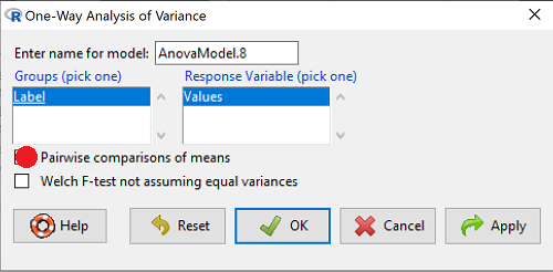
Figure 2. Select Tukey posthoc tests with the one-way ANOVA

R output follows. There’s a lot, but much of it is repeat information. Take your time, here we go.

.Pairs <- glht(AnovaModel.4, linfct = mcp(Label = "Tukey"))
summary(.Pairs) # pairwise tests
     Simultaneous Tests for General Linear Hypotheses
Multiple Comparisons of Means: Tukey Contrasts
 Fit: aov(formula = Values ~ Label, data = sim.Ch12) 

 Linear Hypotheses: 
                  Estimate Std. Error t value Pr(>|t|)     
 Pop2 - Pop1 == 0   -51.30      18.43  -2.783   0.0405 *   
 Pop3 - Pop1 == 0   -19.40      18.43  -1.052   0.7201     
 Pop4 - Pop1 == 0   200.40      18.43  10.871   <0.001 *** 
 Pop3 - Pop2 == 0    31.90      18.43   1.730   0.3233     
 Pop4 - Pop2 == 0   251.70      18.43  13.654   <0.001 *** 
 Pop4 - Pop3 == 0   219.80      18.43  11.924   <0.001 *** 
 --- 
 Signif. codes:  0 '***' 0.001 '**' 0.01 '*' 0.05 '.' 0.1 ' ' 1 
 (Adjusted p values reported -- single-step method) 

 confint(.Pairs) # confidence intervals 
      Simultaneous Confidence Intervals 

 Multiple Comparisons of Means: Tukey Contrasts 

 Fit: aov(formula = Values ~ Label, data = sim.Ch12) 

 Quantile = 2.6927 
 95% family-wise confidence level 
   
 Linear Hypotheses: 
                  Estimate  lwr       upr       
 Pop2 - Pop1 == 0  -51.3000 -100.9382   -1.6618 
 Pop3 - Pop1 == 0  -19.4000  -69.0382   30.2382 
 Pop4 - Pop1 == 0  200.4000  150.7618  250.0382 
 Pop3 - Pop2 == 0   31.9000  -17.7382   81.5382 
 Pop4 - Pop2 == 0  251.7000  202.0618  301.3382 
 Pop4 - Pop3 == 0  219.8000  170.1618  269.4382

Confidence interval plots, Tukey posthoc

Figure 3. Plot of confidence intervals of Tukey HSD

R Commander includes a default 95% CI plot (Fig. 3). From this graph, you can quickly identify the pairwise comparisons for which 0 (zero, dotted vertical line) is included in the interval, i.e., there is no difference between the means (e.g., Pop1 is different from Pop4, but Pop1 is not different from Pop3).

b. Dunnett’s Test for comparisons against a control group

There are situations where we might want to compare our experimental Populations to one control Population or group. Thus, this is likely a case of planned comparisons.
This is common in medical research where there is a placebo (control pill with no drug) or sham operations (operations where every thing but the critical operation is done).
This is also a common research design in ecological or agricultural research where some animal or plant populations are exposed to an environmental factor (e.g. fertilizer, pesticide, pollutant, competitors, herbivores) and other animal or plant populations are not exposed to these environmental factor.
The difference in the statistical procedure for analyzing this type of research design is that the experimental groups may only be compared to the control group.
This results in fewer comparisons.
The formula is the same as for the Tukey’s Multiple Comparison test, except for the calculation of the SE.

Standard Error is changed by multiplying the MS_Error by 2.

And n is the harmonic mean of the sample sizes of the two groups being compared.

$\begin{align*} q = \frac{\bar{X}_{control}-\bar{X}_{A}}{SE} \end{align*}$

where

$\begin{align*} SE=\sqrt{\frac{2/ MS_{error}}{n}} \end{align*}$

R Commander doesn’t provide a simple way to get Dunnett, but we can get it simply enough if we are willing to write some script. Fortunately (OK, by design!), Rcmdr prints commands.

Look at the Output window from the one-way ANOVA with pairwise comparisons: it provides clues as to how we can modify the mcp command (mcp stands for multiple comparisons).

First, I had run the one-way ANOVA command and noted the model (AnovaModel.3). Second, I wrote the following script, modified from above.

Pairs <- glht(AnovaModel.1, linfct = mcp(Label = c("Pop2 - Pop1 = 0", "Pop3 - Pop1 = 0", "Pop4 - Pop1 = 0")))

where Label is my name for the Factor variable. Note that I specified the comparisons I wanted R to make. When I submit the script, nothing shows up in the Output window because the results are stored in my “Pairs.”

I then need to ask R to provide confidence intervals

confint(Pairs)

R output window

Pairs <- glht(AnovaModel.1, linfct = mcp(Label = c("Pop2 - Pop1 = 0", "Pop3 - Pop1 = 0", "Pop4 - Pop1 = 0"))) 
confint(Pairs) 

Simultaneous Confidence Intervals 

 Multiple Comparisons of Means: User-defined Contrasts 

 Fit: aov(formula = Values ~ Label, data = sim.Ch12) 

 Estimated Quantile = 2.4524 
 95% family-wise confidence level 

 Linear Hypotheses: 
  ...... lwr ....... upr 
 Pop2 - Pop1 == 0  .. -51.3000  . -96.5080  ... -6.0920 
 Pop3 - Pop1 == 0  .. -19.4000  . -64.6080  ... 25.8080 
 Pop4 - Pop1 == 0  .. 200.4000  . 155.1920  .. 245.6080

Look for intervals that include zero, therefore, the group does not differ from the Control group (Pop1). How many groups differed from the Control group?

Alternatively, I may write

Tryme <- glht(AnovaModel.1, linfct = mcp(Label = "Dunnett"))
confint(Tryme)

It’s the same (in fact, the default mcp test is the Dunnett).

Tryme <- glht(AnovaModel.1, linfct = mcp(Label = "Dunnett")) 
confint(Tryme) 

Simultaneous Confidence Intervals 

Multiple Comparisons of Means: Dunnett Contrasts 

Fit: aov(formula = Values ~ Label, data = sim.Ch12) 

Estimated Quantile = 2.4514 
95% family-wise confidence level 

Linear Hypotheses: 
Estimate lwr upr 
Pop2 - Pop1 == 0 -51.3000 -96.4895 -6.1105 
Pop3 - Pop1 == 0 -19.4000 -64.5895 25.7895 
Pop4 - Pop1 == 0 200.4000 155.2105 245.5895

Note: Use relevel() command* to set the order of levels in the data set. By default Dunnett procedure in mcp assumes the first level of the factor is the control or reference level. R sorts levels alphabetically, so clearly one option is to always provide a sort-friendly name for the reference level. Naturally, R has you covered if you need to specify a different level as the reference, the relevel() command. For example, instead of Pop1, set reference to Pop2 as follows:

Level 
[1] Pop1 Pop2 Pop3 Pop4
Levels: Pop1 Pop2 Pop3 Pop4

Set new order

Level <- relevel(Level, ref = "Pop2"); Level
[1] Pop1 Pop2 Pop3 Pop4
Levels: Pop2 Pop1 Pop3 Pop4

relevel() works only on unordered factors; if you get this error message it just means you need to specify your character variable as a factor. As you may recall, to confirm a character variable is factor

is.factor(Level)
[1] TRUE

If FALSE, then set character variable to factor.

Level <- as.factor(Level)

* Yes, you could change the order any way you want with level(). For example,

Level <- factor(Level, levels = c("Pop2", "Pop4", "Pop1", "Pop3")); Level

returns

[1] Pop1 Pop2 Pop3 Pop4
Levels: Pop2 Pop4 Pop1 Pop3

c. Bonferroni t

The Bonferroni t test is a popular tool for conducting multiple comparisons. This, too, is consistent with an unplanned comparisons approach. The rationale for this particular test is that the MS_error is a good estimate of the pooled variances for all groups in the ANOVA.

$\begin{align*} Bonferroni = \frac{\bar{X}_{B}-\bar{X}_{A}}{\sqrt{MS_{error}\left ( \frac{1}{n_{B}}+\frac{1}{n_{A}} \right )}} \end{align*}$

and DF = N – k.

Note that in order to achieve a Type I error rate of 5% for all tests, you must divide the 0.05 by the number of comparisons conducted.

Thus, for k = 4 groups,

$\binom{4}{2} = \frac{4!}{2!\left ( k-2 \right )!}$

Here’s a simplified version if you prefer to get all pairwise tests

$\binom{4}{2} = \frac{4!}{2!\left ( k-2 \right )!}$

Use this information then to determine how many total comparisons will be made, then if necessary, use to adjust Type I error rate for one test (the exerimentwise error rate).

For our example, is 0.05/6 = 0.00833. Thus, for a difference between two means to be statistically significant, the P-value must be less than 0.00833.

For Bonferroni, we will use the following script.

Set up one-way ANOVA model (ours has been saved as AnovaModel.1),
Collect all pairwise comparisons with the mcp(~"Tukey") stored in a vector (I called mine Whynot),
and finally, get the Bonferroni adjusted test of the comparisons with the summary command, but addtest = adjusted("bonferroni").

It’s a bit much, but we end up with a very nice output to work with.

Whynot <- glht(AnovaModel.3, linfct = mcp(Label = "Tukey")) 
summary(Whynot, test = adjusted("bonferroni")) 

 Simultaneous Tests for General Linear Hypotheses

Multiple Comparisons of Means: Tukey Contrasts

Fit: aov(formula = Values ~ Label, data = sim.Ch12)

Linear Hypotheses:
Estimate Std. Error t value Pr(>|t|) 
Pop2 - Pop1 == 0 -51.30 18.43 -2.783 0.0512 . 
Pop3 - Pop1 == 0 -19.40 18.43 -1.052 1.0000 
Pop4 - Pop1 == 0 200.40 18.43 10.871 3.82e-12 ***
Pop3 - Pop2 == 0 31.90 18.43 1.730 0.5527 
Pop4 - Pop2 == 0 251.70 18.43 13.654 5.33e-15 ***
Pop4 - Pop3 == 0 219.80 18.43 11.924 2.77e-13 ***
  --- 
 Signif. codes: 0 '***' 0.001 '**' 0.01 '*' 0.05 '.' 0.1 ' ' 1 
 (Adjusted p values reported -- bonferroni method)

Questions

Be able to define and contrast experiment-wise and family-wise error rates.
Read and interpret R output
1. Refer back to the Tukey HSD output. Among the four populations, which pairwise groups were considered “statistically significant” following use of the Tukey HSD?
2. Refer back to the Dunnett’s output. Among the four populations, which population was taken as the control group for comparison?
3. Refer back to the Dunnett’s output. Which pairwise groups were considered “statistically significant” from the control group?
4. Refer back to the Bonferroni output. Among the four populations, which pairwise groups were considered “statistically significant” following use of the Bonferroni correction?
5. Compare and contrast interpretation of results for posthoc comparisons among the four populations based on the three different posthoc methods
Be able to distinguish when Tukey HSD and Dunnet’s post hoc tests are appropriate.
Some microarray researchers object to use of Bonferroni correction because it is too “conservative.” In the context of statistical testing, what errors are the researchers talking about when they say the correction is “conservative.”

Data set used in this page

Label	Value
Pop1	105
Pop1	132
Pop1	156
Pop1	198
Pop1	120
Pop1	196
Pop1	175
Pop1	180
Pop1	136
Pop1	105
Pop2	100
Pop2	65
Pop2	60
Pop2	125
Pop2	80
Pop2	140
Pop2	50
Pop2	180
Pop2	60
Pop2	130
Pop3	130
Pop3	95
Pop3	100
Pop3	124
Pop3	120
Pop3	180
Pop3	80
Pop3	210
Pop3	100
Pop3	170
Pop4	310
Pop4	302
Pop4	406
Pop4	325
Pop4	298
Pop4	412
Pop4	385
Pop4	329
Pop4	375
Pop4	365

R code # copy the data from the full table to clipboard and paste between the double quotes in text=””)

sim.ch12 <- read.table(header=TRUE, sep=",",text="")

#check the dataframe
head(sim.ch12)

Chapter 12 contents

12.1 – The need for ANOVA

Introduction
The multiple comparison problem
Corrections to account for the multiple comparisons problem
ANOVA is a solution
Questions
Data used in this page
Chapter 12 contents

Introduction

Moving from an experiment with two groups to multiple groups is deceptively simple: we move from one comparison to multiple comparisons. Consider an experiment in which we have randomly assigned patients to receive one of three doses of a statin drug (lower cholesterol), including a placebo (eg, Tobert and Newman 2015). Thus, we have three groups or levels of a single treatment factor and we’ll want to test the null hypothesis that the group (level) means are all equal as opposed to the alternative hypothesis in which one or more of the group means, eg, group A, Group B, group C, are different.

$\begin{align*} H_{0}: \bar{X}_{A} = \bar{X}_{B} = \bar{X}_{C} \end{align*}$

The correct procedure is to analyze multiple levels of a single treatment with a one-way analysis of variance followed by a suitable post-hoc (“after this”) test. Two common post-hoc tests are Tukey’s range test (aka Tukey’s HSD [honestly significant difference] test), which is for all pairwise comparisons, or the Dunnett’s test, which compares groups against the control group. Post-hoc tests are discussed in Chapter 12.6.

Note. To get the number of pairwise comparisons $C$ of $k$ observations, let

$\begin{align*} C = \frac{k\left ( k-1 \right )}{2} \end{align*}$

for more on pairwise comparisons, see 10.1 – Compare two independent sample means

For our three group experiment, how many pairwise comparisons can be tested? Therefore, $k = 3$ , and we have

$\begin{align*} C = \frac{3\left ( 3-1 \right )}{2} = 3 \end{align*}$

Thus, for our three groups, A, B, and C, there are three possible pairwise comparisons.

$\begin{align*} H_{1}: \bar{X}_{A} = \bar{X}_{B}\\ H_{2}: \bar{X}_{A} = \bar{X}_{C}\\ H_{3}: \bar{X}_{B} = \bar{X}_{C} \end{align*}$

How many pairwise comparisons for a four group experiment? Check your work, you should get $C = 6$ .

The multiple comparison problem

Let’s say that we’re stubborn. We could do many single two-sample t-tests — certainly, your statistical software won’t stop you — this is a situation that calls for statistical reasoning. Here’s why we should not: we will increase the probability of rejecting a null hypothesis when the null hypothesis is true (eg, discussion in Jafari and Ansari-Pour 2019). That is, the chance we will commit a Type I error increases if we do not account for the lack of independence in these sets of pairwise tests evaluated by t-tests. This is multiplicity or the multiple comparison problem.

Review: when we perform a two-sample t-test we are willing to reject a true null hypothesis 5% of the time. This is what is meant by setting the critical probability value (alpha) = 0.05. By “willing” we mean that we know that our conclusions could be wrong because we ar3 working with samples, not the entire population. (Of course at the time, we have no way of actually knowing WHEN we are wrong, but we do want to know how likely we could be wrong!) However, if we compare three population means we have three separate null hypotheses.

H_O: one or more of the means are different.

But if we conduct these as separate independent sample t-tests, then we are implicitly making the following null hypothesis statements:

$\begin{align*} H_{1}: \bar{X}_{O} = \bar{X}_{B}\\ H_{2}: \bar{X}_{O} = \bar{X}_{C}\\ H_{3}: \bar{X}_{O} = \bar{X}_{C} \end{align*}$

Thus, we have a 5% chance of being wrong for the first hypothesis and/or a 5% chance of being wrong for the second hypothesis and/or a 5% chance of being wrong for the third hypotheses. The chance that we will be wrong for at least one of these hypotheses must now be greater than 5%.

For three separate hypotheses there is a 14% chance of being wrong when we have the probability value for each individual t-test set at α = 0.05. How did we get this result? The point is that these tests are not independent, they are done on the same data set, therefore you can’t simply apply the multiplication probability rule.

Here’s how to figure this: for the set of three hypotheses, the probability of incorrectly rejecting at least one of the null hypotheses is

$\begin{align*} 1 - 0.953 = 0.14 \end{align*}$

So, for three t-tests on the same experiment, the Type I error overall tests (experiment-wise) is actually 14% not 5%. It gets worse as the number of combinations (groups and therefore hypotheses) increases. For four groups, Type I error is actually

$\begin{align*} 1 - 0.956 = 0.265 \end{align*}$

That’s 26.5%, not 5%.

If we have just five populations means to compare the probability of rejecting a null hypothesis when it is true climbs to 60%! How did this happen? The probability or correctly rejecting all of them is now

$\begin{align*} 0.9510 = 0.599 \end{align*}$

So, the probability of incorrectly rejecting one test (Type I error) is now

$\begin{align*} 1 - 0.9510 = 0.401 \end{align*}$

instead of the 5% we think we are testing.

The key argument for why you must use ANOVA to analyze multiple samples instead of a combination of t-tests!! ANOVA guarantees that the overall error rate is the specified 5%.

Why is the Type I error not 5% for each test? Because we conducted ONE experiment, we can conduct only ONE test (we could be right, we could be wrong 5% of the time). If we conduct the experiment over again, on new subjects, each time resulting in new and therefore independent data sets, then Type I error = 5% for each of these independent experiments.

Now, I hope I have introduced you to the issue of Type I error at the level of a single comparison and the idea of an experiment, holding Type I error-rates at 5% across all hypotheses to be evaluated in an experiment. You may wonder why anyone would make this mistake now. Actually, people make this “mistake” all the time and in some fields like evaluating gene expression for microarray data, this error was the norm, not the exception (see for example discussion of this in Jeanmougin et al 2010).

To conclude, if one does multiple tests on the same experiment, whether it is t-tests or some other test for that matter, then our subsequent tests are related. This is what we mean by independence in statistics — and there are many ways that nonindependence may occur in experimental research. For example, we introduced the concept of pseudoreplication, when observations are treated as if they are independent, but they are not (see Chapter 5.2). The “multiple comparison problem” specifically refers to the lack of independence when all the data set from a single experiment is parsed into lots of separate tests. Philosophically, there must be a logical penalty — and that is reflected in the increase in Type I error.

Clearly something must be done about this!

Corrections to account for the multiple comparisons problem

The family-wise (aka experiment-wise) error rate for multiple comparisons is kept at 5%, and each individual-wise comparison is compared against a more strict (i.e., smaller Type I error rate). Put another way, the family-wise error rate is the chance of a number of false positives: making a mistake when we consider many tests simultaneously. The simplest correction for the individual-wise error rate is the Bonferroni correction: test each individual comparison at Type I error equal to $\alpha \slash C$ , where C is the number of comparisons. The Šidák correction, $1-(1-\alpha)^\frac{1}{C}$ , and the Holm-Bonferroni method are alternatives with reportedly better statistical properties (eg, reduced Type II error rates; Ludbrook 1998, Sauder and DeMars 2019).

ANOVA is a solution

One possible solution for getting the correct experiment-wise error rate: adjust for differences in probability for multiple comparisons with the t-test. We used post-hoc tests presented above: you could evaluate the tests after accounting for the change in Type I error. This is what is done in many cases. For example, in genomics. In the early days of gene expression profiling by microarray, it was common to see researchers conduct t-tests for each gene. Since microarrays can have thousands of genes represented on the chip, then these researchers were conducting thousands of t-tests, arranging the t-tests by P-value and counting the number of P-values less than 5% and declaring that the differences were statistically significant.

This error didn’t stand long, and there are now many options available to researchers to handle the “multiple comparisons” problem (some probably better than others, research on this very much an ongoing endeavor in biostatistics). The Bonferroni correction was an available solution, largely replaced by the Holm (aka Holm-Bonferroni) method (Holm 1979). Recall that the Bonferroni correction judged individual p-values statistically significant only if they were less than $\alpha \slash C$ , where, again, α is the family-wise error rate (eg, α = 5%) and C was the number of comparisons. The Holm method orders the C p-values from lowest to highest rank. The method then evaluates lowest p-value, if less than $\alpha \slash C$ , then reject hypothesis for that comparison. Proceed to next p-value, if less than $\alpha \slash C$ , then reject hypothesis for that comparison, and so on until no more comparisons are less than $\alpha \slash C$ .

A MUCH better alternative is to perform a single analysis that takes the multiple-comparisons problem into account: Single Factor ANOVA, also called the one-way ANOVA, plus the post-hoc tests with error correction. We introduce one-way ANOVA in the next section. Post-hoc tests are discussed in Chapter 12.6.

Questions

You should be able to define and distinguish how Bonferoni correction, Dunnett’s test, and Tukey’s test methods protect against inflation of Type I error.
What will be the experiment-wise error rate for an experiment in which there are only two treatment groups?
Experiment-wise error rate may also be called _______________ error rate.
List and compare the three described posthoc approaches to correct for multiple comparison problem,
Glycophosphate-tolerant soy bean is the number one GMO (genetically modified organism) crop plant worldwide. Glycophosphate is the chief active ingredient in Roundup, the most widely used herbicide. A recent paper examined “food quality” of the nutrient and elemental composition of plants drawn from fields which grow soy by organic methods (no herbicides or pesticides) and GMO plants subject to herbicides and pesticides. A total of 28 individual t-tests were used to compare the treatment groups for different levels of nutrients and elements (eg, vitamins, amino acids, etc.,); the authors concluded that 10 of these t-tests were statistically significant at Type I error rate of 5%. Discuss the approach to statistical inference by the authors of this report; include correct use of the terms experiment-wise and individual-wise in your response and suggest an alternative testing approach if it is appropriate in your view.
In a comparative study about resting metabolic rate for eleven species of mammals, how many pairwise species comparisons can the study test?
In Chapter 4.2 we introduced a data set from an experiment. The experiment looked at DNA damage quantified by measuring qualities in a Comet Assay including the Tail length, the percent of DNA in the tail, and olive moment. The data set is copied to end of this page. In the next chapter I’ll ask you to conduct the ANOVA on this experiment. For now, answer the following questions.
a. What is the response variable?
b. Explain why there is only one response variable.
c. How many treatment variables are there?
d. Why is this an ANOVA problem? Include as part of your explanation a statement of the null hypothesis.

Data used in this page

comet assay dataset

Treatment	Tail	TailPercent	OliveMoment*
Copper-Hazel	10	9.7732	2.1501
Copper-Hazel	6	4.8381	0.9676
Copper-Hazel	6	3.981	0.836
Copper-Hazel	16	12.0911	2.9019
Copper-Hazel	20	15.3543	3.9921
Copper-Hazel	33	33.5207	10.7266
Copper-Hazel	13	13.0936	2.8806
Copper-Hazel	17	26.8697	4.5679
Copper-Hazel	30	53.8844	10.238
Copper-Hazel	19	14.983	3.7458
Copper	11	10.5293	2.1059
Copper	13	12.5298	2.506
Copper	27	38.7357	6.9724
Copper	10	10.0238	1.9045
Copper	12	12.8428	2.5686
Copper	22	32.9746	5.2759
Copper	14	13.7666	2.6157
Copper	15	18.2663	3.8359
Copper	7	10.2393	1.9455
Copper	29	22.6612	7.9314
Hazel	8	5.6897	1.3086
Hazel	15	23.3931	2.8072
Hazel	5	2.7021	0.5674
Hazel	16	22.519	3.1527
Hazel	3	1.9354	0.271
Hazel	10	5.6947	1.3098
Hazel	2	1.4199	0.2272
Hazel	20	29.9353	4.4903
Hazel	6	3.357	0.6714
Hazel	3	1.2528	0.2506

Data set, comet assay. Rat lung cells treated with Hazel tea extract and exposed to copper metal. Tail refers to length of the comet tail, TailPercent is percent DNA damage in tail, and OliveMoment refers to Olive's (1990), defined as the fraction of DNA in the tail multiplied by tail length