6.11 – F distribution
Introduction
The F distribution is the probability distribution associated with the F statistic and named in honor of R. A. Fisher. The F distribution is used as the null distribution of the ANOVA test statistic. The F distribution is the ratio of two chi-square distributions, with degrees of freedom v1 and v2 for numerator and denominator, respectively.
We can for illustration purposes define the F statistic as a ratio of two variances,

The F statistic has two sets of degrees of freedom, one for the numerator and one for the denominator. The actual formula for the F distribution is quite complicated and in general we don’t use the F distribution in a way that involves parameter estimation. Rather, it is used in evaluating the statistical significance of the F statistic. Therefore, we produce but a few graphs and a table of critical values to illustrate the distribution.
We call the result of this calculation the F test statistic. We evaluate how often that value or greater of a test statistic will occur by applying the F distribution function. A few graphs to get a sense of what the distribution looks like for varying v1, v2 held to ten degrees of freedom (Fig. 1).
Figure 1. Animated GIF plot of F distribution value for range of degrees of freedom.
By convention in the Null Hypothesis Significance Testing protocol (NHST), we compare the test statistic to a critical value. The critical value is defined as the value of the test statistic that occurs at the Type I error rate, which is typically set to 5%., per our presentations in Chapter 6.7, 6.9, and 6.10. The justification for NHST approach to testing of statistical significance is developed in Chapter 8.
Table of Critical values of the F distribution, one tail (upper)
Degrees of freedom v1 = 1 – 4, v2 = 10
| Fv1, 10 | α = 0.05 | α = 0.025 | α = 0.01 |
| 1 | 4.964 | 6.937 | 10.044 |
| 2 | 4.103 | 5.456 | 7.559 |
| 3 | 3.708 | 4.826 | 6.552 |
| 4 | 3.478 | 4.468 | 5.994 |
For the complete F table see Appendix 20.4
χ2, t and F distributions are related
χ2, t and F distributions are all distributions indexed by their degrees of freedom. With some algebra, these three distributions can be shown to be related to each other. The probabilities tabled in the chi-squared are part of the F-distribution.
Some interesting relationships between the F distribution and other distributions can be shown. By definition we claimed that the F distribution is built on ratio of chi-square distributions, so that should indicate to you the relationship between the two kinds of continuous probability distributions. However, one can also show relationships to other distributions for the F distribution. For example, for the case of v1 = 1 and v2 = any value, then F1,v2 = t2, where t refers to the t distribution.
Questions
- What happens to the shape of the F distribution as degrees of freedom are increased from 1 to 5 to 20 to 100?
- In Rcmdr, which option do you select to get the critical value for df1 = 1 and df=20 at alpha = 5%?
A. F quantiles
B. F probabilities
C. Plot of F distribution
D. Sample from F distribution
Be able to answer these questions using the F table, Appendix 20.4, or using Rcmdr
- For probability α = 5%, and numerator degrees of freedom equal to 1, what is the critical value of the F distribution (upper tail) for 1 degree of freedom? For 5 df? For 20 df? For 30 df?
- The value of the F test statistic is given as 12. With 3 degrees of freedom for the numerator, and ten degrees of freedom for the denominator, what is the approximate probability of this value, or greater from the F distribution?
Chapter 6 contents
- Introduction
- Some preliminaries
- Ratios and proportions
- Combinations and permutations
- Types of probability
- Discrete probability distributions
- Continuous distributions
- Normal distribution and the normal deviate (Z)
- Moments
- Chi-square distribution
- t distribution
- F distribution
- References and suggested readings
6.9 – Chi-square distribution
Introduction
As noted earlier, the normal deviate or Z score can be viewed as randomly sampled from the standard normal distribution. The chi-square distribution describes the probability distribution of the squared standardized normal deviates with degrees of freedom, df, equal to the number of samples taken. (The number of independent pieces of information needed to calculate the estimate, see Ch. 8.) We will use the chi-square distribution to test statistical significance of categorical variables in goodness of fit tests and contingency table problems.
The equation of the chi-square is

where k is the number of groups or categories, from 1 to k, and fi is the observed frequency and fi “hat” is the expected frequency for the kth category. We call the result of this calculation the chi-square test statistic. We evaluate how often that value or greater of a test statistic will occur by applying the chi-square distribution function. Graphs to show chi-square distribution for degrees of freedom equal to 1 – 5, 10, and 20 (Fig. 1).
Figure 1. Animated GIF of plots of chi-square distribution over range of degrees of freedom.
Note that the distribution is asymmetric, particularly at low degrees of freedom. Thus tests using the chi-square are one-tailed (Fig. 2).
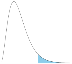
Figure 2. The test of the chi-square is typically one-tailed. In this case, probability of values greater than the critical value.
By convention in the Null Hypothesis Significance Testing protocol (NHST), we compare the test statistic to a critical value. The critical value is defined as the value of the test statistic — the cutoff boundary between statistical significance and insignificance — that occurs at the Type I error rate, which is typically set to 5%. The interpretation of the result is as follows: after calculating a test statistic, we can judge significance of the results relative to the null hypothesis expectation. If our test statistics is greater than the critical value, then the p-value of our results are less than 5% (R will report an exact p-value for the test statistic). You are not expected to be able to follow this logic just yet — rather, we teach it now as a sort of mechanical understanding to develop in the NHST tradition. The justification for this approach to testing of statistical significance is developed in Chapter 8. A portion of the critical values of the chi-square distribution are shown in Figure 3.

Figure 3. Portion of the table of some critical values of chi-square distribution, one tailed (right-tailed or “upper” portion of distribution).
See Appendix for a complete chi-square table.
Example
Professor Hermon Bumpus of Brown University in Providence, Rhode Island, received 136 House Sparrows (Passer domesticus) after a severe winter storm 1 February 1898. The birds were collected from the ground; 72 of the birds survived, 64 did not (Table 1). Bumpus made several measures of morphology on the birds and the data set has served as a classical example of Natural Selection (Chicago Field Museum). We’ll look at this data set when we introduce Linear Regression.
Table 1. Survival statistics of Bumpus House sparrows
| Yes | No | |
| Female | 21 | 28 |
| Male | 51 | 36 |
Was there a survival difference between male and female House Sparrows? This is a classic contingency table analysis, something we will at length in Chapter 9. For now, we report the Chi-square test statistic for this test was 3.1264 and the test had one degree of freedom. What is the critical value of the chi-square distribution at 5% and one degree of freedom?. Typically we would simply use R to look this up
qchisq(c(0.05), df=1, lower.tail=FALSE)
But we can also get this from the table of critical values (Fig. 4). Simply select the row based on the degrees of freedom for the test then scan to the column with the appropriate significance level, again, typically 5% (0.05).

Figure 4. Portion of the chi-square distribution which shows how to find critical value of the chi-square distribution.
For 1 degree of freedom at 5% significance, the critical value is 3.841. Back to our hypothesis: Did male and female survival differ in the Bumpus data set? Following the NHST logic, if the test statistic value (e.g., 3.1264) is greater than the critical value (3.841), then we would reject the null hypothesis. For this example, we would conclude no statistical difference between male and female survival because the test statistic was smaller than the critical value. How likely are these results due to chance? That’s where the p-value comes in. Our test statistic value falls between 5% and 10% (2.706 < 3.1264 < 3.841). In order to get the actual p-value of our test statistic we would need to use R.
R code
Given a chi-square test statistic you can use R to calculate the probability of that value against the null hypothesis. At the R prompt
pchisq(c(3.1264), df=1, lower.tail=FALSE)
And R output
[1] 0.07703368
Because we are using R Commander, simply select the command by following the menu options.
Rcmdr: Distributions → Continuous distributions → Chi-squared distribution → Chi-squared probabilities …
Enter the chi-square value and degrees of freedom (Fig. 5).

Figure 5. Screenshot of input box in Rcmdr for Chi-square probability values.
Questions
- What happens to the shape of the chi-square distribution as degrees of freedom are increased from 1 to 5 to 20 to 100?
Be able to answer these questions using the Chi-square table, Appendix 20.2, or using Rcmdr
- For probability α = 5%, what is the critical value of the chi-square distribution (upper tail)?
- The value of the chi-square test statistic is given as 12. With 3 degrees of freedom, what is the approximate probability of this value, or greater from the chi-square distribution?
Chapter 6 contents
- Introduction
- Some preliminaries
- Ratios and proportions
- Combinations and permutations
- Types of probability
- Discrete probability distributions
- Continuous distributions
- Normal distribution and the normal deviate (Z)
- Moments
- Chi-square (Χ2) distribution
- t distribution
- F distribution
- References and suggested readings