12.2 – One way ANOVA

Introduction
Three important terms you’ll need for one-way ANOVA
Note on experimental design
ANOVA sources of variation
Mean squares
Worked example with R
Questions
Data set
Chapter 12 contents

Introduction

In ANalysis Of VAriance, or ANOVA for short, we likewise have tools to test the null hypothesis of no difference between between categorical independent variables — often called factors when there’s just a few levels to keep track of — and a single, dependent response variable. But now, the response variable is quantitative, not qualitative like the $\chi^2$ tests.

Analysis of variance, ANOVA, is such an important statistical test in biology that we will take the time to “build it” from scratch. We begin by reminding you of where you’ve been with the material.

We already saw an example of this null hypothesis. When there’s only one factor (but with two or more levels), we call the analysis of means and “one-way ANOVA.” In the independent sample t-test, we tested whether two groups had the same mean. We made the connection between the confidence interval of the difference between the sample means and whether or not it includes zero (i.e., no difference between the means). In ANOVA, we extend this idea to a test of whether two or more groups have the same mean. In fact, if you perform an ANOVA on only two groups, you will get the exact same answer as the independent two-sample t-test, although they use different distributions of critical values (t for the t-test, F for the ANOVA — a nice little fact for you square the t-test statistic, you’ll get the F-test statistic: $t^{2} = F$ ).

Let’s say we have an experiment where we’ve looked at the effect of different three different calorie levels on weight change in middle-aged men.

I’ve created a simulated dataset which we will use in our ANOVA discussions. The data set is available at the end of this page (scroll down or click here).

We might graph the mean weight changes ( $\pm$ SEM); Below are two possible outcomes of our experiment (Fig. 1).

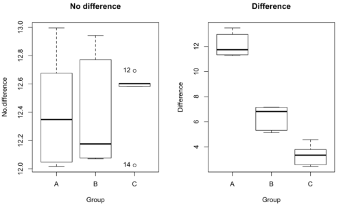
Figure 1. Hypothetical results, box plots.

Figure 1. Hypothetical results of an experiment, box plots. Left, no difference among groups; Right, large differences among groups.

As statisticians and scientists, we would first calculate an overall or grand mean for the entire sample of observations; we know this as the sample mean whose symbol is $\bar{X}$ . But this overall mean is made up of the average of the sample means. If the null hypothesis is true, then the all of the sample means all estimate the overall mean. Put another way, being a member of a treatment group doesn’t matter, i.e., there is no systematic effect, all differences among subjects are due to random chance.

$\begin{align*} H_{0} : \bar{X} = \bar{X}_{A} = \bar{X}_{B} = \bar{X}_{C} \end{align*}$

The hypotheses among are three groups or treatment levels then are:

$\begin{align*} H_{0} : \bar{X}_{A} = \bar{X}_{B} = \bar{X}_{C}&& \end{align*}$

Null that there are no differences among the group means. And the alternative hypotheses include any (or all) of the following possibilities

$\begin{align*} H_{0} : \bar{X}_{A} \ne \bar{X}_{B} = \bar{X}_{C} \end{align*}$

or maybe

$\begin{align*} H_{0} : \bar{X}_{A} = \bar{X}_{B} \ne \bar{X}_{C} \end{align*}$

or… have we covered all possible alternate outcomes among three groups?

In either case, we could use one-way ANOVA to test for “statistically significant differences.”

Three important terms you’ll need for one-way ANOVA

FACTOR: We have one factor of interest. For example, a factor of interest might be

Diet fed to hypertensive subjects (men and women)
Distribution of coral reef sea cucumber species in archipelagos
Antibiotic drug therapy for adolescents with Acne vulgaris (click see Webster 2002 for review).

Note 1: Character vs factor. In R programming, while it is true that a treatment variable can be a character vector like Gender*, such vectors are handled by R as string. In contrast, by claiming Gender as a factor, R handles the variable as a nominal data type. Hence, ANOVA and other GLM functions expect any treatment variable to be declared as a factor:

Gender <- c("Gender non-conforming", "Men", "Non-binary", "Transgender", "Women", "Declined"); Gender
[1] "Gender non-conforming" "Men" "Non-binary" "Transgender" 
[5] "Women" "Declined"

# it’s a string vector, not a factor

is.factor(Gender)
[1] FALSE

Change string vector to a factor.

Gender <- as.factor(Gender); is.factor(Gender) [1] TRUE

* For discussions of ethics of language inclusivity and whether or not such information should be gathered, see Henrickson et al 2020.

LEVELS: We can have multiple levels (2 or more) within the single factor. Some examples of levels for the Factors listed:

Three diets (DASH), diet rich in fruits & vegetables, control diet)
Five archipelagos (Hawaiian Islands, Line Islands, Marshal Islands, Bonin Islands, and Ryukyu Islands)
Five antibiotics (ciprofloxacin, cotrimoxazole, erythromycin, doxycycline, minocycline).

RESPONSE: There is one outcome or measurement variable. This variable must be quantitative (i.e., on the ratio or interval scale). Continuing our examples then

Reduction in systolic pressure
Numbers of individual sea cucumbers in a plot
number of microcomedo.

Note 2: A comedo is a clogged pore in the skin; a microcomedo refers to the small plug. Yes, I had to look that up, too.

The response variable can be just about anything we can measure, but because ANOVA is a parametric test, the response variable must be normally distributed!

Note on experimental design

As we discuss ANOVA, keep in mind we are talking about analyzing results from an experiment. Understanding statistics, and in particular ANOVA, informs how to plan an experiment. The basic experimental design is called a completely randomized experimental design, or CDR, where treatments are assigned to experimental units at random.

In this experimental design, subjects (experimental units) must be randomly assigned to each of these levels of the factor. That is, each individual should have had the same probability of being found in any one of the levels of the factor. The design is complete because randomization is conducted for all levels, all factors.

Thinking about how you would describe an experiment with three levels of some treatment, we would have

Table 1. Summary statistics of three levels for some ratio scale response variable.

Level 1

$\bar_{X}_{1}$

sample mean₁

$s_{1}$

sample standard deviation₁

Level 2

$\bar_{X}_{2}$

sample mean₂

$s_{2}$

sample standard deviation₂

Level 3

$\bar_{X}_{3}$

sample mean₃

$s_{3}$

sample standard deviation₃

Note 3: Table 1 is the basis for creating the box plots in Figure 1.

ANOVA sources of variation

ANOVA works by partitioning total variability about the means (the grand mean, the group means). We will discuss the multiple samples and how the ANOVA works in terms of the sources of variation. There are two “sources” of variation that can occur:

Within Group Variation
Among Groups Variation

So let’s look first at the variability within groups, also called the Within Group Variation.

Consider and experiment to see if DASH diet reduces systolic blood pressure in USA middle-aged men and women with hypertension (Moore et al 2001). After eight weeks we have

We get the corrected sum of squares, SS, for within group

$\begin{align*} within-groups \ SS = \sum_{i=1}^{k}\left [ \sum_{j=1}^{n_{i}}\left ( X_{ij}-\bar{X}_{i} \right )^2 \right ] \end{align*}$

and the degrees of freedom, DF, for within groups

$\begin{align*} within-groups \ DF = \sum_{i=1}^{k}\left ( n_{i}-1 \right ) = N - k \end{align*}$

where i is the identity of the groups, $X_{ij}$ is the individual observations within group i, $\bar{X}_{i}$ is the group i mean, n_i is the sample size within each group, N is the total sample size of all subjects for all groups, and k is the number of groups.

Importantly, this value is also referred to as “error sums of squares” in ANOVA. It’s importance is as follows — In our example, the within group variability would be zero if and only if all subjects within the same diet lost exactly the same amount of weight. This is hardly ever the case of course in a real experiment. Because there are almost always some other unknown factors or measurement error that affect the response variable, there will be some unknown variation among individuals who received the same treatment (within the same group). Thus, the error variance will generally be larger than zero.

The first point to consider: your ANOVA will never result in statistical differences among the groups if the error variance is greater than the second type of variability, the variability between groups.

The second type of variability in ANOVA is that due to the groups or treatments. Individuals given a calorie-restricted diet will loose some weight; individuals allowed to eat a calorie-rich diet likely will gain weight, therefore there will be variability (a difference) due to the treatment. So we can calculate the variability among groups. We get the corrected sum of squares for among groups

$\begin{align*} among-groups \ SS = \sum_{i=1}^{k}n_{i}\left ( X_{i}-\bar{X}\right )^2 \end{align*}$

and the degrees of freedom for among groups

$\begin{align*} among-groups \ DF = k - 1 \end{align*}$

where i is the identity of the groups, $\bar{X}$ is the grand mean as defined in Measures of Central Tendency (Chapter 3.1), $\bar{X}_{i}$ is the group i mean, n_i is the sample size within each group, N is the total sample size of all subjects for all groups, and k is the number of groups.

The sums of squares here is simply subtracting the mean of each population from the overall mean.

If the Factor is not important in explaining the variation among individuals then all the population means will be similar and the sums of squares among populations would be small.
If the Factor is important in explaining some of the variation among the individuals then all the population means will NOT be the same and the sums of squares among populations would be large.

Finally, we can identify the total variation in the entire experiment. We have the total sum of squares.

$\begin{align*} Total \ SS = among-groups \ SS + within-groups \ SS \end{align*}$

Thus, the insight of ANOVA is that variation in the dataset may be attributed to a portion explained by differences among the groups and differences among individual observations within each group. The inference comes from recognizing that if the among group effect is greater than the within group effect, then there will be a difference due to the treatment levels.

Mean squares

To decide whether the variation associated with the among group differences are greater than the within group variation, we calculate ratios of the sums of squares. These are called Mean Squares or MS for short. The ratio of the Mean Squares is called F, the test statistic for ANOVA.

For the one-way ANOVA we will have two Mean Squares and one F, tested with degrees of freedom for both the numerator $MS_{groups}$ , and denominator $MS_{error}$ ).

The Mean Square for (among) groups is

$\begin{align*} MS_{group} = \frac{among-groups \ SS}{among-groups \ DF} \end{align*}$

The Mean Square for error is

$\begin{align*} MS_{error} = \frac{within-groups \ SS}{within-groups \ DF} \end{align*}$

And finally, the value for F, the test statistic for ANOVA, is

$\begin{align*} F = \frac{MS_{group}}{MS_{error}} \end{align*}$

Worked example with R

A factor with three levels, A, B, and C

group <- c("A", "A", "A", "B", "B", "B", "C", "C", "C")

and their responses, simulated

response <- c(10.8, 11.8, 12.8, 6.5, 7, 8, 3.8, 2.8, 3)

We create a data frame

all <- data.frame(group, response)

Of course, you could place the data into a worksheet and then import the worksheet into R. Regardless, we now have our dataset.

Now, call the ANOVA function, aov, and assign the results to an object (e.g., Model.1)

Model.1 <- aov(response ~ group, data=all)

Now, visualize the ANOVA table

summary(Model.1)

and the output from R, the ANOVA table, is shown below

Note 4: Rcmdr: Statistics → Means → One-way ANOVA… see figures 2 and 3 below

Table 2. Output from aov() command, the ANOVA table, for the “Difference” outcome variable.

           Df   Sum Sq    Mean Sq   F value       Pr(>F) 
group       2   111.16      55.58     89.49    0.0000341 ***
Residuals   6     3.73       0.62
---
Signif. codes: 0 '***' 0.001 '**' 0.01 '*' 0.05 '.' 0.1 ' ' 1

Let’s take the ANOVA table one row at a time

The first row has subject headers defining the columns.
The second row of the table “groups” contains statistics due to group, and provides the comparisons among groups.
The third row, “Residuals” is the error, or the differences within groups.

Moving across the columns, then, for each row, we have in turn,

the degrees of freedom (there were 3 groups, therefore 2 DF for group),
the Sums of Squares, the Mean Squares,
the value of F, and finally,
the P-value.

R provides a helpful guide on the last line of the ANOVA summary table, the “Signif[icance] codes,” which highlights the magnitude of the P-value.

What to report? ANOVA problems can be much more complicated than the simple one-way ANOVA introduced here. For complex ANOVA problems, report the ANOVA table itself! But for the one-way ANOVA it would be sufficient to report the test statistic, the degrees of freedom, and the p-value, as we have in previous chapters (e.g., t-test, chi-square, etc.). Thus, we would report:

F = 89.49, df = 2 and 6, p = 0.0000341

where F = 89.49 is the test statistic, df = 2 (degrees of freedom for the among group mean square) and 6 (degrees of freedom for the within group mean square), and p = 0.0000341 is the p-value.

In Rcmdr, the appropriate command for the one-way ANOVA is simply

Rcmdr: Statistics → Means

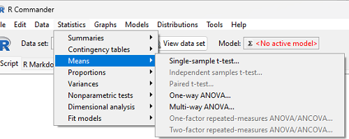
Screenshot Rcmdr select one-way ANOVA

Figure 2. Screenshot Rcmdr select one-way ANOVA

which brings up a simple dialog. R Commander anticipates factor (Groups) and Response variable. Optional, choose Pairwise comparisons of means for post-hoc test (Tukey’s) and, if you do not want to assume equal variances (see Chapter 13), select Welch F-test.

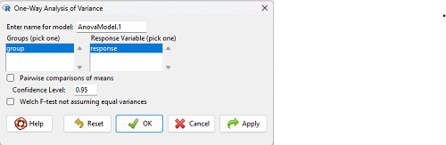
Screenshot Rcmdr select one-way ANOVA options

Figure 3. Screenshot Rcmdr select one-way ANOVA options.

Questions

1. Review the example ANOVA Table and confirm the following

How many levels of the treatment were there?
How many sampling units were there?
Confirm the calculation of $MS_{group}$ and $MS_{error}$ using the formulas contained in the text.
Confirm the calculation of F using the formula contained in the text.
The degrees of freedom for the F statistic in this example were 2 and 6 (F_2,6). Assuming a two-tailed test with Type I error rate of 5%, What is the critical value of the F distribution (see Appendix 20.4)

2. Repeat the one-way ANOVA using the simulated data, but this time, calculate the ANOVA problem for the “No.difference” response variable.

3. Leaf lengths from three strains of Arabidopsis thaliana plants grown in common garden are shown in Fig. 2. Data are provided for you in the following R script.

arabid <- c("wt","wt","wt","AS1","AS1","AS1","AS2","AS2","AS2")
leaf <- c(4.909,5.736,5.108,6.956,5.809,6.888,4.768,4.209,4.065)
leaves <- data.frame(arabid,leaf)

Write out a null and alternative hypotheses
Conduct a test of the null hypothesis by one-way ANOVA
Report the value of the test statistic, the degrees of freedom, and the P-value
Do you accept or reject the null hypothesis? Explain your choice.

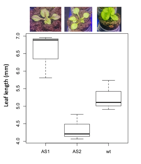
Box plot of length of leaves from three strains of Arabidopsis thaliana

Figure 4. Box plot of lengths of leaves of a 10-day old plant from on of three strains of Arabidopsis thaliana.

4. Return to your answer to question 7 from Chapter 12.1 and review your answer and modify as appropriate to correct your language to that presented here about factors and levels.

5. Conduct the one-way ANOVA test on the Comet assay data presented question 7 from Chapter 12.1. Data are copied for your convenience to end of this page. Obtain the ANOVA table and report the value of the test statistics, degrees of freedom, and p-value.
a. Based on the ANOVA results, do you accept or reject the null hypothesis? Explain your choice.

Data used in this page

Difference, no difference

Table 12.2 Difference or No Difference

Group	No.difference	Difference
A	12.04822	11.336161
A	12.67584	13.476142
A	12.99568	12.96121
A	12.01745	11.746712
A	12.34854	11.275492
B	12.17643	7.167262
B	12.77201	5.136788
B	12.07137	6.820242
B	12.94258	5.318743
B	12.0767	7.153992
C	12.58212	3.344218
C	12.69263	3.792337
C	12.60226	2.444438
C	12.02534	2.576014
C	12.6042	4.575672

Simulated data

Comet assay, antioxidant properties of tea

Data presented in Chapter 12.1

Chapter 12 contents

9 – Inferences, Categorical Data

Introduction
Two kinds of chi-square analyses
Chapter 9 contents

Introduction

No doubt you have already been introduced to chi-square ( $\chi^{2}$ ) tests (click here correct pronounciation), particularly if you’ve had a genetics class, but perhaps you were not told why you were using the $\chi^{2}$ test, as opposed to some other test, for example t-test, ANOVA, or linear regression.

Chi-square analyses are used in situations of discrete (i.e., categorical or qualitative) data types. When you can count the number of “yes” or “no” outcomes from an experiment, then you are talking about a $\chi^{2}$ problem. In contrast, continuous (i.e., quantitative) data types for outcome variables would require you to use the t-test (for two groups) or the ANOVA-like procedures (for two or more groups). Chi-square tests can be applied when you have two or more treatment groups.

Two kinds of chi-square analyses

(1) We ask about the “fit” of our data against predictions from theory. This is the typical chi-square that student’s have been exposed to in biology lab. If outcomes of an experiment can be measured against predictions from some theory, then this is a goodness of fit (gof) $\chi^{2}$ . Goodness of fit is introduced in Ch09.1.

Note 1: The fit concept in statistics is simply how well a statistical model explains the data. As we go forward, this concept will appear frequently.

(2) We ask whether the outcomes of an experiment are associated with a treatment. These are called contingency table problems, and they will be the subject of the next lecture. The important distinction here is that there exists no outside source of information (“theory”) available to make predictions about what we would expect. Contingency tables are introduced in Ch09.2.

Chapter 9 contents

8.1 – The null and alternative hypotheses

Introduction
Statistical Inference in the NHST Framework
NHST Workflow
Null hypothesis
Alternative hypothesis
Alternative hypothesis often may be the research hypothesis
How to interpret the results of a statistical test
Outcomes of an experiment
Questions
Chapter 8 contents

Introduction

Classical statistical parametric tests — t-test (one sample t-test, independent sample-t-test), analysis of variance (ANOVA), correlation, and linear regression— and nonparametric tests like $\chi^{2}$ (chi-square: goodness of fit and contingency table ), share several features that we need to understand. It’s natural to see all the details as if they are specific to each test, but there’s a theme that binds all of the classical statistical inference in order to make claim of “statistical significance.”

a calculated test statistic
degrees of freedom associated with the calculation of the test statistic
a probability value or p-value which is associated with the test statistic, assuming a null hypothesis is “true” in the population from which we sample.
- Recall from our previous discussion (Chapter 8.2) that this is not strictly the interpretation of p-value, but a short-hand for how likely the data fit the null hypothesis. P-value alone can’t tell us about “truth.”
in the event we reject the null hypothesis, we provisionally accept the alternative hypothesis.

Statistical Inference in the NHST Framework

By inference we mean to imply some formal process by which a conclusion is reached from data analysis of outcomes of an experiment. The process at its best leads to conclusions based on evidence. In statistics, evidence comes about from the careful and reasoned application of statistical procedures and the evaluation of probability (Abelson 1995).

Formally, statistics is rich in inference process (Bzdok et al, 2018). We begin by defining the classical frequentist, aka Neyman-Pearson approach, to inference, which involves the pairing of two kinds of statistical hypotheses: the null hypothesis (H_O) and the alternate hypothesis (H_A). The null hypothesis assumes that any observed difference between the groups are the results of random chance (introduced in Ch 2.3 – A brief history of (bio)statistics ), where “random chance” implies that outcomes occur without order or pattern (Eagle 2021). Whether we reject or accept the null hypothesis — a short-hand for the more appropriate “provisionally reject” in light of the humility that our results may reflect a rare sampling event — based on the outcome of our statistical inference, the inference is evaluated against a decision criterion (cf discussion in Christiansen 2005), a fixed statistical significance level (Lehmann 1992). Significance level refers to the setting of a p-value threshold before testing is done. The threshold is often set to Type I error of 5% (Cowles & Davis 1982), but researchers should always consider whether this threshold is appropriate for their work (Benjamin et al 2017).

This inference process is referred to as Null Hypothesis Significance Testing, NHST. Additionally, a probability value will be obtained for the test outcome or test statistic value. In the Fisherian likelihood tradition, the magnitude of this statistic value can be associated with a probability value, the p-value, of how likely the result is given the null hypothesis is “true”. (Again, keep in mind that this is not strictly the interpretation of p-value, it’s a short-hand for how likely the data fit the null hypothesis. P-value alone can’t tell us about “truth”, per our discussion, Chapter 8.2.)

Note 1: About -logP. P-values are traditionally reported as a decimal, like 0.000134, in the closed (set) interval (0,1) — p-values can never be exactly zero or one. The smaller the value, the less the chance our data agree with the null prediction. Small numbers like this can be confusing, particularly if many p-values are reported, like in many genomics works, e.g., GWAS studies. Instead of reporting vanishingly small p-values, studies may report the negative log₁₀ p-value, or -logP. Instead of small numbers, large numbers are reported, the larger, the more against the null hypothesis. Thus, our p-value becomes 3.87 -logP.

R code

-1*log(0.000134,10)
[1] 3.872895

Why log₁₀ and not some other base transform? Just that log₁₀ is convenience — powers of 10.

The antilog of 3.87 returns our p-value

> 10^(-1*3.872895)
[1] 0.0001340001

For convenience, a partial p-value -logP transform table

P-value	-logP
0.1	1
0.01	2
0.001	3
0.0001	4

On your own, complete the table up to -logP 5 – 10. See Question 7 below.

NHST Workflow

We presented in the introduction to Chapter 8 without discussion a simple flow chart to illustrate the process of decision (Figure 1). Here, we repeat the flow chart diagram and follow with descriptions of the elements.

NHST decision flow chart

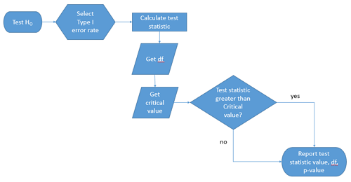
Figure 1. Flow chart of inductive statistical reasoning.

What’s missing from the flow chart is the very necessary caveat that interpretation of the null hypothesis is associated with two kinds of error, Type I error and Type II error. These points and others are discussed in the following sections.

We start with the hypothesis statements. For illustration we discuss hypotheses in terms of comparisons involving just two groups, also called two sample tests. One sample tests in contrast refer to scenarios where you compare a sample statistic to a population value. Extending these concepts to more than two samples is straight-forward, but we leave that discussion to Chapters 12 – 18.

Null hypothesis

By far the most common application of the null hypothesis testing paradigm involves the comparisons of different treatment groups on some outcome variable. These kinds of null hypotheses are the subject of Chapters 8 through 12.

The Null hypothesis (H_O) is a statement about the comparisons, e.g., between a sample statistic and the population, or between two treatment groups. The former is referred to as a one tailed test whereas the latter is called a two-tailed test. The null hypothesis is typically “no statistical difference” between the comparisons.

For example, a one sample, two tailed null hypothesis.

$\begin{align*} H_{0}: \bar{X} = \mu \end{align*}$

and we read it as “there is no statistical difference between our sample mean and the population mean.” For the more likely case in which no population mean is available, we provide another example, a two sample, two tailed null hypothesis.

$\begin{align*} H_{A}: \bar{X}_{1} = \bar{X}_{2} \end{align*}$

Here, we read the statement as “there is no difference between our two sample means.” Equivalently, we interpret the statement as both sample means estimate the same population mean.

$\begin{align*} H_{A}: \bar{X}_{1} = \bar{X}_{2} = \mu \end{align*}$

Under the Neyman-Pearson approach to inference we have two hypotheses: the null hypothesis and the alternate hypothesis. The hull hypothesis was defined above.

Note 2: Tails of a test are discussed further in chapter 8.4.

Alternative hypothesis

Alternative hypothesis (H_A): If we conclude that the null hypothesis is false, or rather and more precisely, we find that we provisionally fail to reject the null hypothesis, then we provisionally accept the alternative hypothesis. The view then is that something other than random chance has influenced the sample observations. Note that the pairing of null and alternative hypotheses covers all possible outcomes. We do not, however, say that we have evidence for the alternative hypothesis under this statistical regimen (Abelson 1995). We tested the null hypothesis, not the alternative hypothesis. Thus, it is incorrect to write that, having found a statistical difference between two drug treatments, say aspirin and acetaminophen for relief of migraine symptoms, it is not correct to conclude that we have proven the case that acetaminophen improves improves symptoms of migraine sufferers.

For the one sample, two tailed null hypothesis, the alternative hypothesis is

$\begin{align*} H_{A}: \bar{X}\neq \mu \end{align*}$

and we read it as “there is a statistical difference between our sample mean and the population mean.” For the two sample, two tailed null hypothesis, the alternative hypothesis would be

$\begin{align*} H_{A}: \bar{X}_{1}\neq \bar{X}_{2} \end{align*}$

and we read it as “there is a statistical difference between our two sample means.”

Alternative hypothesis often may be the research hypothesis

It may be helpful to distinguish between technical hypotheses, scientific hypothesis, or the equality of different kinds of treatments. Tests of technical hypotheses include the testing of statistical assumptions like normality assumption (see Chapter 13.3) and homogeneity of variances (Chapter 13.4). The results of inferences about technical hypotheses are used by the statistician to justify selection of parametric statistical tests (Chapter 13). The testing of some scientific hypothesis like whether or not there is a positive link between lifespan and insulin-like growth factor levels in humans (Fontana et al 2008), like the link between lifespan and IGFs in other organisms (Holtzenberger et al 2003), can be further advanced by considering multiple hypotheses and a test of nested hypotheses and evaluated either in Bayesian or likelihood approaches (Chapter 16 and Chapter 17).

How to interpret the results of a statistical test

Any number of statistical tests may be used to calculate the value of the test statistic. For example, a one sample t-test may be used to evaluate the difference between the sample mean and the population mean (Chapter 8.5) or the independent sample t-test may be used to evaluate the difference between means of the control group and the treatment group (Chapter 10). The test statistic is the particular value of the outcome of our evaluation of the hypothesis and it is associated with the p-value. In other words, given the assumption of a particular probability distribution, in this case the t-distribution, we can associate a probability, the p-value, that we observed the particular value of the test statistic and the null hypothesis is true in the reference population.

By convention, we determine statistical significance (Cox 1982; Whitley & Ball 2002) by assigning ahead of time a decision probability called the Type I error rate, often given the symbol α (alpha). The practice is to look up the critical value that corresponds to the outcome of the test with degrees of freedom like your experiment and at the Type I error rate that you selected. The Degrees of Freedom (DF, df, or sometimes noted by the symbol v), are the number of independent pieces of information available to you. Knowing the degrees of freedom is a crucial piece of information for making the correct tests. Each statistical test has a specific formula for obtaining the independent information available for the statistical test. We first were introduced to DF when we calculated the sample variance with the Bessel correction, n – 1, instead of dividing through by n. With the df in hand, the value of the test statistic is compared to the critical value for our null hypothesis. If the test statistic is smaller than the critical value, we fail to reject the null hypothesis. If, however, the test statistic is greater than the critical value, then we provisionally reject the null hypothesis. This critical value comes from a probability distribution appropriate for the kind of sampling and properties of the measurement we are using. In other words, the rejection criterion for the null hypothesis is set to a critical value, which corresponds to a known probability, the Type I error rate.

Before proceeding with yet another interpretation, and hopefully less technical discussion about test statistics and critical values, we need to discuss the two types of statistical errors. The Type I error rate is the statistical error assigned to the probability that we may reject a null hypothesis as a result of our evaluation of our data when in fact in the reference population, the null hypothesis is, in fact, true. In Biology we generally use Type I error α = 0.05 level of significance. We say that the probability of obtaining the observed value AND H_O is true is 1 in 20 (5%) if α = 0.05. Put another way, we are willing to reject the Null Hypothesis when there is only a 5% chance that the observations could occur and the Null hypothesis is still true. Our test statistic is associated with the p-value; the critical value is associated with the Type I error rate. If and only if the test statistic value equals the critical value will the p-value equal the Type I error rate.

The second error type associated with hypothesis testing is, β, the Type II statistical error rate. This is the case where we accept or fail to reject a null hypothesis based on our data, but in the reference population, the situation is that indeed, the null hypothesis is actually false.

Thus, we end with a concept that may take you a while to come to terms with — there are four, not two possible outcomes of an experiment.

Outcomes of an experiment

What are the possible outcomes of a comparative experiment\? We have two treatments, one in which subjects are given a treatment and the other, subjects receive a placebo. Subjects are followed and an outcome is measured. We calculate the descriptive statistics aka summary statistics, means, standard deviations, and perhaps other statistics, and then ask whether there is a difference between the statistics for the groups. So, two possible outcomes of the experiment, correct\? If the treatment has no effect, then we would expect the two groups to have roughly the same values for means, etc., in other words, any difference between the groups is due to chance fluctuations in the measurements and not because of any systematic effect due to the treatment received. Conversely, then if there is a difference due to the treatment, we expect to see a large enough difference in the statistics so that we would notice the systematic effect due to the treatment.

Actually, there are four, not two, possible outcomes of an experiment, just as there were four and not two conclusions about the results of a clinical assay. The four possible outcomes of a test of a statistical null hypothesis are illustrated in Table 1.

Table 1. When conducting hypothesis testing, four outcomes are possible.

		H_O in the population
		True	False
Result of statistical test	Reject H_O	Type I error with probability equal to α (alpha)	Correct decision, with probability equal to 1 – β (1 – beta)
Result of statistical test	Fail to reject the H_O	Correct decision with probability equal to 1 – α (1 – alpha)	Type II error with probability equal to β (beta)

In the actual population, a thing happens or it doesn’t. The null hypothesis is either true or it is not. But we don’t have access to the reference population, we don’t have a census. In other words, there is truth, but we don’t have access to the truth. We can weight, assigned as a probability or p-value, our decisions by how likely our results are given the assumption that the truth is indeed “no difference.”

If you recall, we’ve seen a table like Table 1 before in our discussion of conditional probability and risk analysis (Chapter 7.3). We made the point that statistical inference and the interpretation of clinical tests are similar (Browner and Newman 1987). From the perspective of ordering a diagnostic test, the proper null hypothesis would be the patient does not have the disease. For your review, here’s that table (Table 2).

Table 2. Interpretations of results of a diagnostic or clinical test.

		Does the person have the disease\?
		Yes	No
Result of the diagnostic test	Positive	sensitivity of the test (a)	False positive (b)
Result of the diagnostic test	Negative	False negative (c)	specificity of the test (d)

Thus, a positive diagnostic test result is interpreted as rejecting the null hypothesis. If the person actually does not have the disease, then the positive diagnostic test is a false positive.

Questions

Match the corresponding entries in the two tables. For example, which outcome from the inference/hypothesis table matches specificity of the test\?
Find three sources on the web for definitions of the p-value. Write out these definitions in your notes and compare them.
In your own words distinguish between the test statistic and the critical value.
Can the p-value associated with the test statistic ever be zero\? Explain.
Since the p-value is associated with the test statistic and the null hypothesis is true, what value must the p-value be for us to provisionally reject the null hypothesis\?
All of our discussions have been about testing the null hypothesis, about accepting or rejecting, provisionally, the null hypothesis. If we reject the null hypothesis, can we say that we have evidence for the alternate hypothesis\?
What are the p-values for -logP of 5, 6, 7, 8, 9, and 10\? Complete the p-value -logP transform table.
Instead of log₁₀ transform, create a similar table but for negative natural log transform. Which is more convenient? Hint: log(x, base=exp(1))

Chapter 8 contents

Introduction
The null and alternative hypotheses
The controversy over proper hypothesis testing
Sampling distribution and hypothesis testing
Tails of a test
One sample t-test
Confidence limits for the estimate of population mean
References and suggested readings