9.5 – Fisher exact test
Introduction
We mentioned that chi-square tests for contingency tables are fine as long as two conditions are met. These are the assumptions of a  test.
test.
- No cell should have expected values less than 5%.
- The test performs poorly at DF = 1 because we are approximating an infinite distribution with an exact test.
You will note that any time you have a 2X2 table, the second condition is always an issue because 2X2 tables have DF=1. Thus, in biomedical research, it is common to have an experiment that may be appropriate for a contingency analysis but the data may suffer from one or both of these limitations. Fisher’s exact test is always an option for these types of problems, but with the advantage that it always returns the exact p-value.
A reminder, the 2×2 table looks like
Table 1. 2×2 table reporting numbers of subjects who have (Yes) or do not have (No) the event.
| Column 1 | Column 2 | ||
| Subjects | Yes | No | |
| Row 1 | Treatment 1 | a | b |
| Row 2 | Treatment 2 | c | d |
where a is the count of Treatment 1 – treated subjects who have the event, b is the count of Treatment 1 – treated subjects who do not have the event, c is the count of Treatment 2 – treated subjects who have the event, d is the count of Treatment 2 – treated subjects who do not have the event. Note the row and column totals:

For example, a fairly common, “Gee, that’s curious,” fact is the seven left-handed US Presidents since 1901 (21), is higher than the proportion of left-handers in the general population (about 10%). For comparison, we could ask the same question about Vice Presidents.†
Table 2. U.S. Presidents and Vice-Presidents handedness.
| Subjects | Yes | No |
| Presidents | 7 | 14 |
| Vice presidents | 5 | 20 |
†Seven Vice-Presidents went on to become President, four right-handers, three left-handers.
Ronald A. Fisher came up with a test that is now called “Fisher’s Exact test” that circumvents this problem. It is an extremely useful test to know about because it provides a way to get an exact probability of the outcome compared to all other possible outcomes. Thus, when asked for a possible alternate to the chi-square contingency test for a 2X2 table, you can respond “Fisher’s Exact test.”
Although tedious to calculate by hand, and resource demanding when done by computer because of the multiple factorial expressions, the major advantage of the test is that it does not rely on the assumption that an underlying distribution applies. The Fisher Exact test can be used to calculate the exact probability of the observed outcome (P).
The equation for the Fisher Exact test can be written as

where R stands for row total, C stands for column total, n is the sample size, ! is the factorial, and a, b, c, and d are defined as in Table 1.
How does Fisher’s Exact test work? The data are setup in the usual way for a contingency problem, but now, we calculate the probability for all possible outcomes that we COULD have seen from our experiment, and ask if the actual outcome is unusual (low p-value). The trick is recognizing that you have to keep the totals constrained (note row and column totals stay the same).
Table 3. Original 2X2 contingency table (bold), with the next two more extreme outcomes.
| original data |  |
more extreme | |
next more extreme still | |
| Yes | No | Yes | No | Yes | No |
| 10 | 5 | 11 | 4 | 12 | 3 |
| 4 | 12 | 3 | 13 | 2 | 14 |
 |
 |
 |
I’ve shown just the one-tailed outcomes, so the p-values are for one-tailed tests of hypothesis. The essence of the test is to find all outcomes MORE extreme than the original, in one direction. The one-tailed P-value then is the sum of all probabilities from those more extreme tables of outcomes.
To get the two-tailed probability, remember that you multiply the one-tailed probability by two. More accurate methods are also available (Agresti 1992).
Calculation of Fisher’s test involves using all possible combinations and factorials. Rcmdr has Fisher’s 2X2 built in via the Contingency table and as part of some Rcmdr plugins (e.g., RcmdrPlugin.EBM, the Evidence Based Medicine plugin). Here we illustrate Fisher Exact test from the context menu in the main Statistics menu.
Alternatively, there are many web sites out there that provide an online calculator for Fisher’s Exact test. Here’s a link to one such calculator on GraphPad’s web site, cookies must be enabled to run this calculator).
To get the Fisher Exact test, your data must already be summarized into a 2X2 table, in which case you can use R Commander via the Contingency tables… menu selection (Fig 1).
Table 4. 2X2 table smokers vs vitamin use.
| Smoker: No | Smoker: Yes | |
| Vitamin use: No | 14 | 26 |
| Vitamin use: Yes | 19 | 15 |
With the data summarized as in Table 4, we can proceed directly via R Commander to analyze the contingency table, either by Chi-square test of Fisher exact test. First, bring up menu to enter the data (Fig 1):
Rcmdr: Statistics → Contingency tables… → Enter and analyze two-way table…
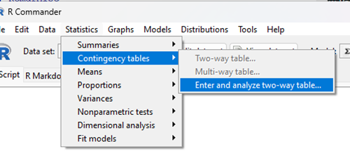
Figure 1. Screenshot Rcmdr menu, Contingency tables.
The image of the R worksheet below contains two columns: Smoker (No, Yes) and Vitamin use (No, Yes). Complete the form (Fig 2).
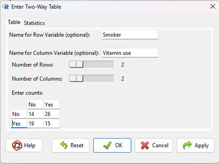
Figure 2. Screenshot Rcmdr menu, Enter Two-Way Table.
Alternatively, if the original data are available, do not tally the counts, let R do the work for you. The worksheet would be stacked like so (Table 5).
Table 5. Portion of subject and row entries in stacked worksheet for smokers vs vitamin use.
| Subject | Vitamin.use | Smoking |
| 1 | No | No |
| 2 | No | No |
| 3 | No | No |
| 4 | No | No |
| 5 | No | No |
| . | . | . |
| 71 | Yes | Yes |
| 72 | Yes | Yes |
| 73 | Yes | Yes |
| 74 | Yes | Yes |
And from the R Commander menu select as before
Rcmdr: Statistics → Contingency tables… → Two way table … (Fig 3).
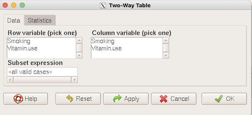
Figure 3. Screenshot Rcmdr two-way table menu, load the data from stacked worksheet.
Data is now ready.
R code
To carry out contingency table analysis on the entered data (Fig 2 or Fig 3), select the Statistics option tab (Fig 4, green arrow).
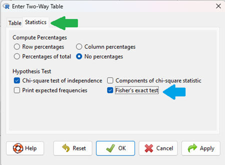
Figure 4. Screenshot Rcmdr menu Statistics option. Select Chi-square test of independence, Fisher’s exact test, or both.
Check the box next to the Fisher’s exact test (Fig 4, blue arrow).
Click OK, and here is the R output.
> fisher.test(.Table)
Fisher's Exact Test for Count Data

data: .Table
p-value = 0.1008
alternative hypothesis: true odds ratio is not equal to 1
95 percent confidence interval:
0.1496417 1.1985775
sample estimates:
odds ratio
0.4302094
We accepted the defaults Is this a one or two-tailed test of hypothesis?
What can we conclude about the null hypothesis? Do we accept or reject?
Want to know what the “odds ratio” is? Follow the link to the next subchapter.
When to use the Fisher Exact Test?
Here’s the take-home message: the Fisher exact test is an alternate and better choice over the contingency table chi-square for 2X2 tables if one or more of the cells has expected values less than 5%. It is also appropriate for cases in which you have only 1 degree of freedom (as do all 2X2 tables!), but it doesn’t make sense if each cell has more than 5% expected values (the calculation is too tedious), but rather, apply the Yate’s correction. As the sample sizes get larger, the different methods converge to virtually identical answers.
Some examples.
Is there an association between final grades and attendance on a randomly selected day?
Table 6. First 2X2 scenario.
| cc | Yes | No |
| Letter grade A | 2 | 3 |
| Other letter grade | 1 | 6 |
Table 7. Second 2X2 scenario.
| cc | Yes | No |
| Letter grade A | 5 | 6 |
| Other letter grade | 2 | 12 |
Table 8. Third 2X2 scenario.
| cc | Yes | No |
| Letter grade A | 10 | 12 |
| Other letter grade | 4 | 24 |
Code hints for tests with direct 2X2 entry with matrix() are
grades.Table <- matrix(c(2,3,1,6), 2, 2, byrow=TRUE)
Chi-square test of independence
chisq.test(grades.Table, correct=FALSE)
Fisher Exact test
fisher.test(grades.Table, alternative = "greater")
Questions
1. Apply Fisher exact test on the four contingency tables (a – d) introduced in section 9.3, question 2. Make note of the p-value from Fisher exact test and from analyses used to complete question 2. Note any trends. (Hint: make sure you are testing the same null hypothesis.)
(a)
| Yes | No | |
| A | 18 | 6 |
| B | 3 | 8 |
(b)
| Yes | No | |
| A | 10 | 12 |
| B | 3 | 14 |
(c)
| Yes | No | |
| A | 5 | 12 |
| B | 12 | 18 |
(d)
| Yes | No | |
| A | 8 | 12 |
| B | 3 | 3 |
Quiz Chapter 9.5
Fisher Exact Test
Chapter 9 contents
9.2 – Chi-square contingency tables
 from a, b, c, and d 2X2 table format formula
 effect size
Introduction
This page covers a lot of ground to extend our discussion of implementations of the chi-square test to experimental data and introduces several related statistics, including a correlation coefficient for categorical data and an introduction to agreement and reliability measurement statistics.
We begin with contingency tables.
We just completed a discussion about goodness of fit tests, inferences on categorical traits for which a theoretical distribution or expectation is available. We offered Mendelian ratios as an example in which theory provides clear-cut expectations for the distribution of phenotypes in the F2 offspring generation. This is an extrinsic model — theory external to the study guides in the calculation of expected values — and it reflects a common analytical task in epidemiology.
But for many other kinds of categorical outcomes, no theory is available. Today, most of us accept the link between tobacco cigarette smoking and lung cancer. The evidence for this link was reported in many studies, some better designed than others.
Consider the famous Doll and Hill (1950) report on smoking and lung cancer. They reported (Table IV Doll and Hill 1950), for men with lung cancer, only two out of 649 were non-smokers. In comparison, 27 case-control patients (ie, patients in the hospital but with other ailments, not lung cancer) were nonsmokers, but 622 were smokers (Table 1).
Table 1. Doll and Hill (1950).
| Smokers | Non-smokers | |
| Lung cancer | 647 | 2 |
| Case controls, no lung cancer | 622 | 27 |
A more recent example from the study of the efficacy of St John’s Wort (Hypericum perforatum) as a treatment for major depression (Shelton et al 2001, Apaydin et al. 2016). Of patients who received St. John’s Wort over 8 weeks, 14 were deemed improved while 98 did not improve. In contrast 5 patients who received the placebo were deemed improved while 102 did not improve (Table 2).
Table 2. St. John’s Wort and depression
| Improved | Not improved | |
| St. John’s Wort | 14 | 98 |
| Placebo | 5 | 102 |
Note 1: The St. John’s Wort problem is precisely a the time to remind any reader of Mike’s Biostatistics Book: under no circumstances is medical advice implied from my presentation. From the National Center for Complementary and Integrative Medicine: “It has been clearly shown that St. John’s wort can interact in dangerous, sometimes life-threatening ways with a variety of medicines.”
These kinds of problems are direct extensions of our risk analysis work in Chapter 7. Now, instead of simply describing the differences between case and control groups by Relative Risk Reduction or odds ratios, we instruct how to do inference on the risk analysis problems.
Thus, faced with absence of coherent theory as guide, the data themselves can be used (intrinsic model), and at least for now, we can employ the test.
Note 2: The preferred analysis is to use a logistic regression approach, Chapter 18.3, because additional covariates can be included in the model.
In this lesson we will learn how to extend the analyses of categorical data to cases where we do not have a prior expectation — we use the data to generate the tests of hypotheses. This would be an intrinsic model. One of the most common two-variable categorical analysis involves 2X2 contingency tables. We may have one variable that is the treatment variable and the second variable is the outcome variable. Some examples provided in Table 3.
Table 3. Some examples of treatment and outcome variables suitable for contingency table analysis.
| Treatment Variable and Levels | Outcome Variable(s) | Reference |
| Lead exposure
Levels: Low, Medium, High |
Intelligence and development | Bellinger et al 1987 |
| Wood preservatives
Levels: Borates vs. Chromated Copper Arsenate |
Effectiveness as fungicide | Hrastnik et al 2013 |
| Antidepressants
Levels: St. John’s Wort, conventional antidepressants, placebo |
Depression relief | Linde et al 2008 |
| Coral reefs
Levels: Protected vs Unprotected |
Fish community structure | Guidetti 2006 |
| Aspirin therapy
Levels: low dose vs none |
Cancer incidence in women | Cook et al 2013 |
| Aspirin therapy
Levels: low dose vs none |
Cancer mortality in women | Cook et al 2013 |
Table 4 were examples of published studies returned from a quick PubMed search; there are many examples (meta-analysis opportunities!). However, while they all can be analyzed by contingency tables analysis, they are not exactly the same. In some cases, the treatments are fixed effects, where the researcher selects the levels of the treatments (see Ch12.3 and Ch14.3 for discussion about fixed vs random effects in experimental design).
In other cases, each of these treatment variables need not be actual treatments (in the sense that an experiment was conducted), but it may be easier to think about these as types of experiments. These types of experiments can be distinguished by how the sampling from the reference population were conducted. Before we move on to our main purpose, to discuss how to calculate contingency tables, I wanted to provide some experimental design context by introducing two kinds of sampling (Chapter 5.5).
Our first kind of sampling scheme is called unrestricted sampling. In unrestricted sampling, you collect as many subjects (observations) as possible, then assign subjects to groups. A common approach would be to sample with a grand total in mind; for example, your grant is limited and so you only have enough money to make 1000 copies of your survey and you therefore approach 1000 people. If you categorize the subjects into just two categories (eg, Liberal, Conservative), then you have a binomial sample. If instead you classify the subjects a number of variables, eg, Liberal or Conservative, Education levels, income levels, homeowners or renters, etc., then this approach is called multinomial sampling. The point in either case is that you have just utilized a multinomial sampling approach. The aim is to classify your subjects to their appropriate groups after you have collected the sample.
Logically what must follow unrestricted sampling would be restricted sampling. Sampling would be conducted with one set of “marginal totals” fixed. Margins refers to either the row totals or to the column totals. The sampling scheme is referred to as compound multinomial. The important distinction from the other two types is that the number of individuals in one of the categories is fixed ahead of time. For example, in order to determine if smoking influences respiratory health, you approach as many people as possible to obtain 100 smokers.
The contingency table analysis
We introduced the 2×2 contingency table (Table 4) in Chapter 7.
Table 4. 2X2 contingency table
| Outcome |
|||
| Exposure or Treatment group | Yes | No | Marginal total |
| Exposure (Treatment) | a | b | Row1 = a + b |
| Nonexposure (Control) | c | d | Row2 = c + d |
| Marginal total | Column1 = a + c |
Column2 = a + c |
N |
Contingency tables are all of the form (Table 5)
Table 5. Basic format of a 2X2 table
| Outcome 1 | Outcome 2 | |
| Treatment 1 | Yes | No |
| Treatment 2 | Yes | No |
Regardless of how the sampling occurred, the analysis of the contingency table is the same; mechanically, we have a chi-square type of problem. In both contingency table and the “goodness of fit” Chi-Square analyses the data types are discrete categories. The difference between GOF and contingency table problems is that we have no theory or external model to tell us about what to expect. Thus, we calculate expected values and the degrees of freedom differently in contingency table problems. To learn about how to perform contingency tables we will work through an example, first the long way, and then using a formula and the a, b, c, and d 2X2 table format. Of course, R can easily do contingency tables calculations for us.
Doctors noticed that a new form of Hepatitis (HG, now referred to as GB virus C), was common in some HIV+ populations (Xiang et al 2001). Accompanying the co-infection, doctors also observed an inverse relationship between HG loads and HIV viral loads: patients with high HG titers often had low HIV levels. Thus, the question was whether co-infection alters the outcome of patients with HIV — do HIV patients co-infected with this HG progress to AIDS and mortality at rates different from non-infected HIV patients? I’ve represented the Xiang et al (2001) data in Table 6.
Table 6. Progression of AIDS for patients co-infected with HG [GB virus C], Xiang et al data (2001)
| Lived | Died | Row totals | |
| HG+ | 103 | 41 | 144 |
| HG- | 95 | 123 | 218 |
| Column totals | 198 | 164 | 362 |
Note 3: HG virus is no longer called a hepatitis virus, but instead is referred to as GB virus C, which, like hepatitis viruses, is in the Flaviviridae virus family. For more about the GB virus C, see review article by Bhattarai and Stapleton (2012).
Our question was: Do HIV patients co-infected with this HG progress to AIDS and mortality at rates different from non-infected HIV patients? A typical approach to analyze such data sets is to view the data as discrete categories and analyze with a contingency table. So we proceed.
Setup the table for analysis
Rules of contingency tables (see Kroonenberg and Verbeek 2018). What follows is a detailed walk through setting up and interpreting a 2X2 table. Note that I maintain our a, b, c, d cell order, with row 1 referencing subjects exposed or part of treatment group and row 2 referencing subjects not exposed (or part of the control group), as introduced in Chapter 7.
The Hepatitis G data from Xiang et al 2001 data, arranged in 2X2 format (Table 7).
Table 7. Format of 2X2 table Xiang et al (2001) dataset.
| Lived | Died | Row totals | |
| HG+ | a | b | a + b |
| HG- | c | d | c + d |
| Column totals | a + c | b + d | N |
The data are placed into the cells labeled a, b, c, and d.
Cell a : The number of HIV+ individuals infected with HG that lived beyond the end of the study.
Cell b : The number of HIV+ individuals infected with HG that died during the study.
Cell c : The number of HIV+ individuals not infected with HG that lived.
Cell d : The number of HIV+ individuals not infected with HG that died.
This is a contingency table because the probability of living or dying for these patients may have been contingent on coinfection with hepatitis G.
State the examined hypotheses
HO: There is NO association between the probability of living and coinfection with hepatitis G.
For a contingency table this means that there should be the same proportion of individuals with and without hepatitis G that either lived or died (1:1:1:1).
Now, compute the Expected Values in the Four cells (a, b, c, d)
- Calculate the Expected Proportion of Individuals that lived in Entire Sample:
Column 1 Total / Total = Expected Proportion of those that lived beyond the study. - Calculate Expected Proportion of Individuals that died in Entire Sample:
Column 2 Total / Total = Expected Proportion that died during the study. - Calculate the Expected Proportion of Individuals that lived and were HG+
Expected Proportion of living (step 1 above) x Row 1 Total = Expected For Cell A. - Calculate the Expected Proportion of Individuals that died and were HG+
Expected Proportion died x Row 1 Total = Expected For Cell B - Calculate the Expected Proportion of surviving individuals that were HG-
Expected Proportion lived x Row 2 Total = Expected For Cell C - Calculate the Expected Proportion of individuals that died that were HG-
Expected Proportion that died x Row 2 Total = Expected For Cell D
Yes, this can get a bit repetitive! But, we are now done — remember, we’re working through this to review how the intrinsic model is applied to obtain expected values.
To summarize what we’ve done so far, we now have
Observations arranged in a 2X2 table
Calculated the expected proportions, ie, the Expected values under the Null Hypothesis.
Now, we proceed to conduct the chi-square test of the null hypothesis — The observed values may differ from these expected values, meaning that the Null Hypothesis is False.
Table 8. Copy Table 6 data set
| Lived | Died | Row totals | |
| HG+ | 103 | 41 | 144 |
| HG- | 95 | 123 | 218 |
| Column totals | 198 | 164 | 362 |
Get the Expected Values
- Calculate the Expected Proportion of Individuals that lived in Entire Sample:
Column 1 Total (198) / Total (362) = 0.5470 - Calculate Expected Proportion of Individuals that died in Entire Sample:
Column 2 Total (164) / Total (362) = 0.4530 - Calculate the Expected Proportion of Individuals that lived and were HG+
Expected Proportion of living (0.547) x Row 1 Total (218) = Cell A = 119.25 - Calculate the Expected Proportion of Individuals that died and were HG+
Expected Proportion died (0.453) x Row 1 Total (218) = Cell B = 98.75. - Calculate the Expected Proportion of surviving individuals that were HG-
Expected Proportion lived (0.547) x Row 2 Total (144) = Cell C = 78.768 - Calculate the Expected Proportion of individuals that died that were HG-
Expected Proportion that died 0(.453) X Row 2 Total = Cell D = 65.232
Thus, we have (Table 9)
Table 9. Expected values for Xiang et al (2001) data set (Table 6 and Table 8)
| Lived | Died | Row totals | |
| HG+ | 78.768 | 65.232 | 144 |
| HG- | 119.25 | 98.75 | 218 |
| Column totals | 198 | 164 | 362 |
Now we are ready to calculate the Chi-Square Value
Recall the formula for the chi-square test

Table 10. Worked contingency table for Xiang et al (2001) data set (Table 6 and Table 8)
| Cell |  |
|
| a | (103 – 87.768)2 = 78.768 | 7.4547 |
| b | (41 – 65.232)2 = 65.232 | 9.002 |
| c | (95 – 119.25)2 = 119.25 | 4.93134 |
| d | (123 – 98.75)2 = 98.75 | 5.95506 |
 |
27.3452 |
Adding all the parts we have the chi-square test statistic  . To proceed with the inference, we test using the chi-square distribution.
Determine the Critical Value of  test and evaluate the null hypothesis
Now recall that we can get the critical value of this test in one of two (related!) ways. One, we could run this through our statistical software and get the p-value, the probability of our result and the null hypothesis is true. Second, we look up the critical value from an appropriate statistical table. Here, we present option 2.
We need the Type I error rate α and calculate the degrees of freedom for the problem. By convention, we set α = 0.05. Degrees of freedom for contingency table is calculated as
Degrees of Freedom = (# rows – 1) x (# columns – 1)
and for our example → DF = (2 – 1) x (2 – 1) = 1.
Note. How did we get the 1 degree of freedom? Aren’t there 4 categories and shouldn’t we therefore have k – 1 = 3 df? We do have four categories, yes, but the categories are not independent. We need to take this into account when we evaluate the test and this lack of independence is accounted for by the loss of degrees of freedom.
What exactly is not independent about our study?
-
- The total number of observations is set in advance from the data collection.
- We also have the column and row totals set in advance. The number of HIV individuals with or without Hepatitis G infection was determined at the beginning of the experiment. The number of individuals that lived or died was also determined before we we conducted the test.
- Then the first cell (let us make that cell A) can still vary anywhere from 0 to N i (sample size of the first drug).
- Once the first cell (A) is determined then the next cell in that row (B) will have to add up to N i.
- Also the other cell in the same column as the first cell (C) must add up to the Column 1 Total.
- Lastly, the last cell (D) must have the Row 1 Total add up to the correct number.
All this translates into there being only one cell that is FREE TO VARY, hence, only one degree of freedom.
Get the Critical Value from a chi-square distribution table: For our example, look up the critical value for DF = 1, α = 0.05, you should get 3.841. The 3.841 is the value of the chi-square we would expect at 5% and the null hypothesis is in fact true condition in the population.
Once we obtain the critical value we simply use the previous statement regarding the probability of the Null Hypothesis being TRUE. We Reject the Null Hypothesis when the calculated test statistic is greater than the Critical Value. We Accept the Null Hypothesis when the calculated is less than the Critical Value. In our example we got 27.3452 for our calculated test statistic, thus we reject the null hypothesis and conclude, that, at least for the sample in this study, there was an association between the probability of patients living past the study period and the presence of hepatitis G.
from a, b, c, and d 2X2 table format formula
If a hand calculation is required, a simpler formula to use is

where N is the sum of all observations in the table, r1 and r2 are the marginal row totals, and c1 and c2 are the marginal column totals from the 2×2 contingency table (eg, Table 4). If you are tempted to try this in a spreadsheet, and assuming your entries for a, b, c, d, and N look like Table 11, then a straightforward interpretation requires referencing five spreadsheet cells no less than 13 times! Not to mention a separate call to the distribution to calculate the p-value (one tailed test).
Note 4: This formulation was provided as equation 1 in Yates 1984 (referred to in Serra 2018), but is likely found in the earlier papers on dating back to Pearson.
Table 11. Example spreadsheet with formulas for odds ratio (OR), Pearson’s , and p-value from distribution.
| A | B | C | D | E | F | G | |
| 1 | |||||||
| 2 | a | 103 | OR | =( 2*5)/(3*4) 2*5)/(3*4) |
|||
| 3 | b | 41 | |||||
| 4 | c | 95 | |||||
| 5 | d | 123 | chisq, p | =(((2*5-3*4)^2)*6)/ (SUM( 2:3)*SUM(4:5)*SUM( 2,4)*SUM(3,5)) |
=CHIDIST(F5,1) | ||
| 6 | N | 632 |
Now, let’s see how easy this is to do in R.
effect size
Inference on hypotheses about association, there’s statistical significance — evaluate p-value compared to Type I error, eg, 5% — and then there’s biological importance, the strength of the association. The concept of effect size is an attempt to communicate the likely importance of a result. Several statistics are available to communicate effect size: for that’s φ, phi for the φ (phi) coefficient.

where N is the total. Phi for our example is

R code
sqrt(27.3452/362)
and R returns
[1] 0.274844
Effect size statistics typically range from 0 to 1; Cohen (1992) suggested the following interpretation
Table 12. Cohen’s interpretation of d values.
| Effect size | Interpretation |
| < 0.2 | Small, weak effect |
| 0.5 | Moderate effect |
| > 0.8 | Large effect |
For our example,  effect size of the association between co-infection with GB virus C and mortality was weak in the patients with HIV infection. The function
 phi() in psych package will calculate phi coefficient from a 2X2 table.
Agreement, kappa, and inter-rater reliability
I imagine by now you have made the leap — can we use the contingency table to assess agreement between (inter-) two judges (raters) who evaluate the same object? A naive approach would be to calculate simple agreement, the percent of objects in the list of items evaluated for which both judges agree (concur). For a binomial Yes or No, then agreement (concordance) occurs when both judges report “Yes,” or both report “No,” displayed on the main diagonal of the 2X2 table. The other possible combinations (Yes vs No and No vs Yes) are disagreement (discordance) and would be displayed on the off-diagonal of the 2X2 matrix.
Unfortunately, simple agreement, while intuitive, cannot discriminate between true agreement and agreement by chance. Cohen’s kappa (Cohen 1960, McHugh 2012) is used to assess agreement, aka inter-rater reliability, for binomial and nominal data types for two judges (raters). Cohen’s 1960 paper has been enormously impactful, with more than 53K citations (Google Scholar, Fall 2024), and spawned a number of additional measures of agreement, eg, weighted kappa for more than binomial levels, Fleiss kappa for three or more raters, ICC for ratio scale, discussed in Ch12.3). It’s beyond the scope of this text to review the context of such terms as agreement, and reliability, for just two terms used to evaluate results from two independent observers of the “same” event or object, and leave that to the reader to confirm how to report such endeavors.
Off we go. Cohen’s kappa is defined as

where po is the proportion in agreement and pc is proportion of agreement expected by chance. Essentially, then, interpretable kappa values fall between 0 and 1 (0% to 100%); negative kappa estimates are possible. Cohen (1960) noted that for kappa to equal 1, the off diagonal elements would all have to be zero.
Cohen provided an estimate of the standard error for kappa as

and 95% confidence intervals are then  .
.
Here, we review calculation of simple agreement and Cohen’s kappa, with just the two levels. Both simple agreement and Cohen’s kappa (κ), are available in R via the icc package. Cohen’s kappa is also available in the psych package, with the cohen.kappa() function providing a confidence interval estimate directly.
Note 5: Base R includes the function kappa(), but that returns an estimate for the condition number of the matrix, or how close to singular the matrix solution may be, ie, determinant is zero and its inverse is unavailable.
Use of both is illustrated here with a simulated coin toss example modified from a nice 2018 summary of Cohen’s kappa at r-bloggers. The R code
library(irr)
# simulate some data
N = 24
flips1 <- rbinom(n = N, size = 1, prob = 0.5)
flips2 <- rbinom(n = N, size = 1, prob = 0.5)
coins<-cbind(flips1, flips2)
Confirm the data set.
head(coins)
flips1 flips2
[1,] 0 1
[2,] 1 0
[3,] 1 0
[4,] 1 1
[5,] 0 0
[6,] 1 0
and create a 2X2 table.
I stacked the data
head(StackedCoin)
Side Coins    HT
1 0 flips1 tails
2 1 flips1 heads
3 1 flips1 heads
4 1 flips1 heads
5 0 flips1 tails
6 1 flips1 heads
then created a simple 2×2 table (see Note 6 below for a simple explanation for why “.Table” as a named object).
.Table <- xtabs(~Coins+HT, data=StackedCoin)
Table 13. coins as 2X2 table.
| tails | heads | |
| flips1 | 10 | 14 |
| flips2 | 14 | 10 |
We can calculate the phi coefficient for Table 13.
phi(.Table, digits = 3)
[1] -0.167
and would conclude no correlation between the two sets of coin tosses.
Now, agreement statistics. Both agree() and kappa2() expect an unstacked (wide) data format. It’s not necessary, but we’ll call a value of 1 as “heads up” and a value of 0 as “tails up” of the tossed coin.
Next, simple agreement.
agree(coins, tolerance=0)
R returns
Subjects = 24
Raters = 2
%-agree = 41.7
Now, a proper agreement statistic.
kappa2(coins)
and R returns
Subjects = 24
Kappa = -0.135
z = -0.7
p-value = 0.484
Results with psych:cohen.kappa, which provides the 95% confidence interval as default output.
Cohen Kappa and Weighted Kappa correlation coefficients and confidence boundaries
                 lower estimate upper
unweighted kappa -0.51    -0.14  0.24
weighted kappa   -0.51    -0.14  0.24
Number of subjects = 24
By chance, the two independent toss of 24 coins had 10 rows of “agreement” (H:H or T:T), simply due to chance. However, results of kappa find no agreement between the two sets of coin tosses.
In summary, we see that simple agreement and the kappa statistic don’t return similar results. Percent agreement reported 41%, whereas kappa was zero. We know percent agreement can’t reflect anything in the coin toss case because each toss is independent from the next. We’ll have you explore repeated trials of coin tosses to help convince you that simple agreement is not a reliable measure of agreement (see question 6 below).
Interpreting agreement values is not straightforward, and some argue agreement statistics should be avoided in favor of disagreement measures (for example, see discussion in Pontius and Millones 2011). Cohen suggested (Table 14)
Table 14. Landis and Koch’s (1977) interpretation of Cohen’s kappa.
| Cohen’s kappa | Agreement? |
| < 0 | none |
| 0.01 — 0.20 | slight |
| 0.21 — 0.40 | fair |
| 0.41 — 0.60 | moderate |
| 0.61 — 0.80 | substantial |
| 0.81 — 1 | nearly perfect |
Note 6: Wikipedia page for Cohen’s kappa suggests that this interpretation began with the Landis and Koch 1997 paper in the journal Biometrics. I haven’t confirmed this — regardless, this paper is also highly influential, with more than 89K citations (Fall 2024).
Even a cursory look at Table 14 should lead to questions about scenarios in which a range of agreement “substantial” would provide little comfort about the agreement between the judges or the reliability of the instrument used, for example forensic cases or histology of tissue biopsies.
Contingency table analyses in Rcmdr
Assuming you have already summarized the data, you can enter the data directly in the Rcmdr contingency table form. If your data are not summarized, then you would use Rcmdr's Two-way table… for this. We will proceed under the assumption that you have already obtained the frequencies for each cell in the table.
Rcmdr: Statistics → Contingency tables → Enter and analyze two-way table…
Here you can tell R how many rows and how many columns (Fig 1).
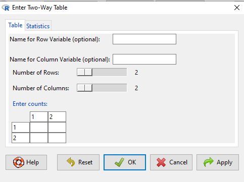
Figure 1. Screenshot R Commander menu for 2X2 data entry with counts.
The default is a 2X2 table. For larger tables, use the sliders to increase the number of rows, columns, or both.
Next, enter the counts. You can edit every cell in this table, including the headers. In the next panel, I will show you the data entry and options. The actual calculation of the test statistic is done when you select the “Chi-square test of independence” check-box (Fig 2).
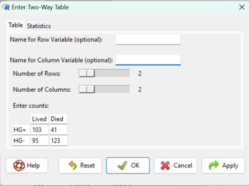
Figure 2. Display of Xiang et al data entered into R Commander menu.
After entering the data, click on the Statistics tab (Fig 3).
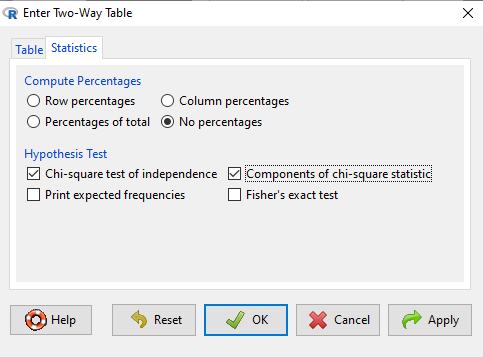
Figure 3. Screenshot Statistics options for contingency table.
If you also select “Components of chi-square statistic” option, then R will show you the contributions of each cell (O-E) towards the chi-square test statistic value. This is helpful to determine if rejection of the null is due to a subset of the categories, and it also forms the basis of the heterogeneity tests, a subject we will pick up in the next section.
Here’s the R output from R Commander. Note the “2, 2, byrow=TRUE” instructions (check out R help to confirm what
.Table <- matrix(c(103,41,95,123), 2, 2, byrow=TRUE)
dimnames(.Table) <- list("rows"=c("HG+", "HG-"), "columns"=c("Lived", "Died"))

.Table # Counts
     columns
rows Lived Died
 HG+   103   41
 HG-   95   123

.Test <- chisq.test(.Table, correct=FALSE)
.Test

Pearson's Chi-squared test

data: .Table
X-squared = 27.339, df = 1, p-value = 0.0000001708

round(.Test$residuals^2, 2) # Chi-square Components
    columns
rows Lived Died
HG+   7.46 9.00
HG-   4.93 5.95

remove(.Test)
remove(.Table)
end R output.
Note 7: R Commander often cleans up after itself by removing objects like .Test and .Table. This is not necessary for the code to work, but does make it easier for you to go back and modify the code without worrying about confusing objects.
Lots of output, take a deep breath and remember… The minimum output we need to look at is… (Table 15)?
Table 15. Minimally expected outcome for report from a statistical test.
| Value of the test statistic | 27.339 |
| Degrees of freedom | 1 |
| p-value | 0.0000001708 |
We can see that the p-value 1.7-7 is much less than Type 1 α = 0.05, thus, by our decision criterion we reject the null hypothesis (provisionally of course, as science goes).
Note 7: Simple enough to get R to report numbers as you need. For example, R code
myNumber = 0.0000001708
format(myNumber, scientific = TRUE, digits=2)
returns
[1] "1.7e-07"
Questions
- Instead of R Commander, try the contingency table problem in R directly.
myData <- matrix(c(103,41,95,123))
chisq.test(myData)
Is this the correct
contingency table analysis? Why or why not? - For many years National Football League games that ended in ties went to “sudden death,” where the winner was determined by the first score in the extra period of play, regardless of whether or not the other team got an opportunity to possess the ball on offense. Thus, in more than 100 games (140), the team that won the coin toss and therefore got the ball first in overtime, won the game following either a kicked field goal or after a touchdown was scored. In 337 other games under this system, the outcome was not determined by who got the ball first. Many complained that the “sudden death” format was unfair and in 2013 the NFL changed its overtime rules. Beginning 2014 season, both teams got a chance to possess the ball in overtime, unless the team that won the coin toss also went on to score a touchdown at which time that team would be declared the winner. In this new era of over-time rules ten teams that won the coin toss went on to score a touchdown in their first possession and therefore win the game, whereas in 54 other overtime games, the outcome was decided after both teams had a chance on offense (data as of 1 December 2015). These data may be summarized in the table
First possession win? Yes No Coin flip years 140 337 New era 10 54 A. What is the null hypothesis?
B. Which is more appropriate: to calculate an odds ratio or to calculate an RRR?
C. This is a contingency table problem. Explain why
D. Conduct the test of the null hypothesis.
E. What is the value of the test statistic? Degrees of freedom? P-value?
F. Evaluate the results of your analysis — do you accept or reject the null hypothesis? - Return to the Doll and Hill (1950) data: 2 men with lung cancer were nonsmokers, 647 men with lung cancer were cigarette smokers. In comparison, 27 case-control patients (ie, patients in the hospital but with other ailments, not lung cancer) were nonsmokers, but 622 were cigarette smokers.
A. What is the null hypothesis?
B. Which is more appropriate: to calculate an odds ratio or to calculate an RRR?
C. This is a contingency table problem. Explain why
D. Conduct the test of the null hypothesis.
E. What is the value of the test statistic? Degrees of freedom? P-value?
F. Evaluate the results of your analysis — do you accept or reject the null hypothesis? - A more recent example from the study of the efficacy of St John’s Wort as a treatment for major depression (Shelton et al 2001). Of patients who received St. John’s Wort over 8 weeks, 14 were deemed improved while 98 did not improve. In contrast 5 patients who received the placebo were deemed improved while 102 did not improve.
A. What is the null hypothesis?
B. Which is more appropriate: to calculate an odds ratio or to calculate an RRR?
C. This is a contingency table problem. Explain why
D. Conduct the test of the null hypothesis.
E. What is the value of the test statistic? Degrees of freedom? P-value?
F. Evaluate the results of your analysis — do you accept or reject the null hypothesis? - Return to the coin toss simulation and repeat comparisons between simple agreement and Cohen’s kappa for different values of N. Do you see any trend(s) for the two measures as sample size increases or decreases?
- Repeat the coin toss simulation for N = 24 up to five times, each time calculate simple agreement and Cohen’s kappa. Provide a table of your five results plus the example, and generalize simple agreement vs Cohen’s kappa as a reliable measure of agreement. Hint: you may want to use Descriptive statistics to help make your case.
Quiz Chapter 9.2
Chi-square contingency tables
Chapter 9 contents
7.4 – Epidemiology: Relative risk and absolute risk, explained
Risk communication.
Epidemiology is the study of patterns of health and illness of populations. An important task in an epidemiology study is to identify risks associated with disease. Epidemiology is a crucial discipline used to inform about possible effective treatment approaches, health policy, and about the etiology of disease.
Please review terms presented in section 7.1 before proceeding. RR and AR are appropriate for cohort-control and cross-sectional studies (see 2.4 and 5.4) where base rates of exposure and unexposed or numbers of affected and non-affected individuals (prevalence) are available. Calculations of relative risk (RR) and relative risk reduction (RRR) are specific to the sampled groups under study whereas absolute risk (AR) and absolute risk reduction (ARR) pertain to the reference population. Relative risks are specific to the study, absolute risks are generalized to the population. Number needed to treat (NNT) is a way to communicate absolute risk reductions.
An example of ARR and RRR risk calculations using natural numbers.
Clinical trials are perhaps the essential research approach (Sibbald and Roland 1998; Sylvester et al 2017); they are often characterized with a binary outcome. Subjects either get better or they do not. There are many ways to represent risk of a particular outcome, but where possible, using natural numbers is generally preferred as a means of communication, particularly to the general public. Consider the following example (pp 34-35, Gigerenzer 2015): What is the benefit of taking a cholesterol-lowering drug, Pravastatin, on the risk of deaths by heart attacks and other causes of mortality? Press releases (e.g., Maugh 1995), from the study stated the following:
“… the drug pravastatin reduced … deaths from all causes 22%”
A subsequent report (Skolbekken 1998) presented the following numbers (Table 1).
Table 1. Reduction in total mortality (5 year study) for people who took Pravastatin compared to those who took placebo.
| Deaths per 1000 people with high cholesterol (> 240 mg/dL) |
No deaths | Cumulative incidence |
||
| Treatment | Pravastatin
(n = 3302) |
a= 32 |
b= 3270 |
CIe |
| Placebo
(n = 3293) |
c= 41 |
d= 3252 |
CIu | |
where cumulative incidence refers to the number of new events or cases of disease divided by the total number of individuals in the population at risk.
Do the calculations of risk
The risk reduction (RR), or the number of people who die without treatment (placebo) minus those who die with treatment (Pravastatin), 

and the cumulative incidence in the exposed (treated) group, CIe, is  , and cumulative incidence in the unexposed (control) group, CIu, is
  . We can calculate another statistic called the risk ratio,

because the risk ratio is less than one, we interpret that statins reduce the risk of mortality from heart attack. In other words, statins lowered the risk by 0.78.
But is this risk reduction meaningful?
Now, consider the absolute risk reduction (ARR) is 
Relative risk reduction, or the absolute risk reduction divided by the proportion of patients who die without treatment, is 
Conclusion: high cholesterol may contribute to increased risk of mortality, but the rate is very low in the population as a whole (the ARR).
Another useful way to communicate benefit is to calculate the Number Needed to Treat (NNT), or the number of people who must receive the treatment to save (benefit) one person. The ideal NNT is a value of one (1), which would be interpreted as everyone improves who receives the treatment. By definition, NNT must be positive; however, a resulting negative NNT would suggest the treatment may cause harm, i.e., number needed to harm (NNH).
For this example, the NNT is

therefore, to benefit one person, 111 need to be treated. The flip side of the implications of NNT, although one person may benefit by taking the treatment, 110 ( ) will take the treatment, but will NOT RECEIVE THE BENEFIT, but do potentially get any side effect of the treatment.
Confidence interval for NNT is derived from the Confidence interval for ARR.
For a sample of 100 people drawn at random from a population (which may number in the millions), then repeat the NNT calculation for a different sample of 100 people, do we expect the first and second NNT estimates to be exactly the same number? No, but we do expect them to be close and we can define what we mean by close as we expect each estimate to be within certain limits. While we expect the second calculation to be close to the first estimate, we would be surprised if it was exactly the same. And so, which is the correct estimate, the first or the second? They both are, in the sense that they both estimate the parameter NNT (a property of a population).
We use confidence interval to communicate where we believe the true estimate for NNT to be. Confidence Intervals (CI) allow us to assign a probability to how certain we are about the statistic and whether it is likely to be close to the true value (Altman 1998, Bender 2001). We will calculate the 95% CI for the ARR using the Wald method, then take the inverse of these estimates for our 95% CI. The Wald method assumes normality.
For CI of ARR, we need sample size for control and treatment groups; like all confidence intervals, we need to calculate the standard error of the statistic, in this, case, the standard error (SE) for ARR is approximately

where SE is the standard error for ARR. For our example, we have

The 95% CI for ARR is approximately 
For the Wald estimate, replace the 2 with  , which comes from the normal table for z at
(why the 2 in the equation? Because it is plus or minus so we divide the frequency 0.95 in half) and for our example, we have 
and the inverse for NNT CI is 
Our example exemplifies the limitation of the Wald approach (cf. Altman 1998): our confidence interval includes zero, and doesn’t even include our best estimate of NNT (111).
Note 1: By now I trust you can see differences for results by direct input of the numbers into R and what you get by the natural numbers approach. In part this is because we round in our natural number calculations — remember, while it makes more sense to communicate about whole numbers (people) and not fractions (fractions of people!), rounding through the calculations adds error to the final value. As long as you know the difference and the relevance between approximate and exact solutions, this shouldn’t cause concern.
Software: epiR.
R has many epidemiology packages, epiR and epitools are two. Most of the code presented stems from epiR.
We need to know about our study design in order to tell the functions which statistics are appropriate to estimate. For our statin example, the design was prospective cohort (i.e., cohort.count in epiR package language), not case-control or cross-sectional (review in Chapter 5.4).
library(epiR)
Table1 <- matrix(c(32,3270,41,3252), 2, 2, byrow=TRUE, dimnames = list(c("Statin", "Placebo"), c("Died", "Lived")))
Table1
        Died Lived
Statin    32  3270
Placebo   41  3252
epi.2by2(Table1, method="cohort.count", outcome = "as.columns")
R output
           Outcome + Outcome - Total           Inc risk *
Exposed +         32      3270  3302 0.97  (0.66 to 1.37)
Exposed -         41      3252  3293 1.25  (0.89 to 1.69)
Total             73      6522  6595 1.11  (0.87 to 1.39)

Point estimates and 95% CIs:
-------------------------------------------------------------------
Inc risk ratio                          0.78 (0.49, 1.23)
Inc odds ratio                          0.78 (0.49, 1.24)
Attrib risk in the exposed *           -0.28 (-0.78, 0.23)
Attrib fraction in the exposed (%)    -28.48 (-103.47, 18.88)
Attrib risk in the population *        -0.14 (-0.59, 0.32)
Attrib fraction in the population (%) -12.48 (-37.60, 8.05)
-------------------------------------------------------------------
Uncorrected chi2 test that OR = 1: chi2(1) = 1.147 Pr>chi2 = 0.284
Fisher exact test that OR = 1: Pr>chi2 = 0.292
Wald confidence limits
CI: confidence interval
* Outcomes per 100 population units
The risk ratio we calculated by hand is shown in green in the R output, along with other useful statistics (see ?epi2x2 for help with these additional terms) not defined in our presentation.
We explain results of chi-square goodness of fit (Ch 9.1) and Fisher exact (Ch 9.5) tests in Chapter 9. Suffice to say here, we interpret the p-value (Pr) = 0.284 and 0.292 to indicate that there is no association between mortality from heart attacks with or without the statin (i.e., the Odds Ratio, OR, not statistically different from one).
Wait! Where’s NNT and other results?
Use another command in epiR package, epi.tests(), to determine the specificity, sensitivity, and positive (or negative) predictive value.
epi.tests(Table1)
and R returns
          Outcome + Outcome - Total
Test +           32      3270  3302
Test -           41      3252  3293
Total            73      6522  6595

Point estimates and 95% CIs:
--------------------------------------------------------------
Apparent prevalence *                    0.50 (0.49, 0.51)
True prevalence *                        0.01 (0.01, 0.01)
Sensitivity *                            0.44 (0.32, 0.56)
Specificity *                            0.50 (0.49, 0.51)
Positive predictive value *              0.01 (0.01, 0.01)
Negative predictive value *              0.99 (0.98, 0.99)
Positive likelihood ratio                0.87 (0.67, 1.13)
Negative likelihood ratio                1.13 (0.92, 1.38)
False T+ proportion for true D- *        0.50 (0.49, 0.51)
False T- proportion for true D+ *        0.56 (0.44, 0.68)
False T+ proportion for T+ *             0.99 (0.99, 0.99)
False T- proportion for T- *             0.01 (0.01, 0.02)
Correctly classified proportion *        0.50 (0.49, 0.51)
--------------------------------------------------------------
* Exact CIs
Additional statistics are available by saving the output from epi2x2() or epitests() to an object, then using summary(). For example save output from epi.2by2(Table1, method="cohort.count", outcome = "as.columns") to object myEpi, then
summary(myEpi)
look for NNT in the R output
$massoc.detail$NNT.strata.wald
       est    lower    upper
1 -362.377 -128.038  436.481
Thus, the NNT was 362 (compared to 111 we got by hand) with 95% Confidence interval between -436 and +128 (make it positive because it is a treatment improvement).
Note 2: Strata (L. layers), refer to subgroups, for example, sex or age categories (see discussion in Ch05.4). Our examples here are not presented as subgroup analysis, but epiR reports by name strata.
epiR reports a lot of additional statistics in the output and for clarity, I have not defined each one, just the basic terms we need for BI311. As always, see help pages (e.g., ?epi.2x2 or ?epitests)for more information about structure of an R command and the output.
We’re good, but we can work the output to make it more useful to us.
Improve output from epiR.
For starters, if we set interpret=TRUE instead of the default, interpret=FALSE, epiR will return a richer response.
fit <- epi.2by2(dat = as.table(Table1), method = "cohort.count", conf.level = 0.95, units = 100, interpret = TRUE, outcome = "as.columns")
fit
R output. In addition to the table of coefficients (above), interpret=TRUE provides more context, shown below
Measures of association strength:
The outcome incidence risk among the exposed was 0.78 (95% CI 0.49 to 1.23) times less than the outcome incidence risk among the unexposed.

The outcome incidence odds among the exposed was 0.78 (95% CI 0.49 to 1.24) times less than the outcome incidence odds among the unexposed.

Measures of effect in the exposed:
Exposure changed the outcome incidence risk in the exposed by -0.28 (95% CI -0.78 to 0.23) per 100 population units. -28.5% of outcomes in the exposed were attributable to exposure (95% CI -103.5% to 18.9%).

Number needed to treat for benefit (NNTB) and harm (NNTH):
The number needed to treat for one subject to be harmed (NNTH) is 362 (NNTH 128 to infinity to NNTB 436).

Measures of effect in the population:
Exposure changed the outcome incidence risk in the population by -0.14 (95% CI -0.59 to 0.32) per 100 population units. -12.5% of outcomes in the population were attributable to exposure (95% CI -37.6% to 8.1%).
That’s quite a bit. Another trick is to get at the table of results. We install a package called broom, which includes a number of ways to handle output from R functions, including those in the epiR package. Broom takes from the TidyVerse environment; tables are stored as tibbles.
library(broom)

# Test statistics
tidy(fit, parameters = "stat")
R output
# A tibble: 3 × 4
term statistic df p.value
<chr> <dbl> <dbl> <dbl>
1 chi2.strata.uncor 1.15 1 0.284
2 chi2.strata.yates 0.909 1 0.340
3 chi2.strata.fisher NA NA 0.292
We can convert the tibbles into our familiar data.frame format, and then select only the statistics we want.
# Measures of association
fitD <- as.data.frame(tidy(fit, parameters = "moa")); fitD
R output, all 15 measures of association!
                  term     estimate     conf.low    conf.high
1       RR.strata.wald    0.7783605    0.4914679   1.23272564
2     RR.strata.taylor    0.7783605    0.4914679   1.23272564
3      RR.strata.score    0.8742994    0.6584540   1.10340173
4       OR.strata.wald    0.7761915    0.4876209   1.23553616
5     OR.strata.cfield    0.7761915           NA           NA
6      OR.strata.score    0.7761915    0.4894450   1.23093168
7        OR.strata.mle    0.7762234    0.4718655   1.26668220
8    ARisk.strata.wald   -0.2759557   -0.7810162   0.22910484
9   ARisk.strata.score   -0.2759557   -0.8000574   0.23482532
10     NNT.strata.wald -362.3770579 -128.0383246 436.48140194
11    NNT.strata.score -362.3770579 -124.9910314 425.84844829
12  AFRisk.strata.wald   -0.2847517   -1.0347210   0.18878949
13  PARisk.strata.wald   -0.1381661   -0.5933541   0.31702189
14  PARisk.strata.piri   -0.1381661   -0.3910629   0.11473067
15 PAFRisk.strata.wald   -0.1248227   -0.3760279   0.08052298
We can call out just the statistics we want from this table by calling to the specific elements in the data.frame (rows, columns).
fitD[c(1,4,7,9,12),]
R output
                 term   estimate   conf.low  conf.high
1      RR.strata.wald  0.7783605  0.4914679  1.2327256
4      OR.strata.wald  0.7761915  0.4876209  1.2355362
7       OR.strata.mle  0.7762234  0.4718655  1.2666822
9  ARisk.strata.score -0.2759557 -0.8000574  0.2348253
12 AFRisk.strata.wald -0.2847517 -1.0347210  0.1887895
Software: epitools.
Another useful R package for epidemiology is epitools, but it comes with it’s own idiosyncrasies. We have introduced the standard 2X2 format, with a, b, c, and d cells defined as in Table 1, above. However, epitools does it differently, and we need to update the matrix. By default, epitools has the unexposed group (control) in the first row and the non-outcome (no disease) is in the first column. To match our a,b,c, and d matrix, use the epitools command to change this arrangement with the rev() argument. Now, the analysis will use the contingency table on the right where the exposed group (treatment) is in the first row and the outcome (disease) is in the first column (h/t M. Bounthavong 2021). Once that’s accomplished, epitools returns what you would expect.
Calculate relative risk
risk1 <- 32 / (3270 + 32)
risk2 <- 41 / (3525 + 41)
risk1 - risk2
and R returns
-0.00180638
odds ratio
library(epitools)
oddsratio.wald(Table1, rev = c("both"))
and R returns
$data
              Outcome
Predictor Disease2 Disease1 Total
 Exposed2      517       36   553
 Exposed1      518       11   529
Total         1035       47  1082

$measure
           odds ratio with 95% C.I.
Predictor   estimate      lower      upper
 Exposed2  1.0000000        NA         NA
 Exposed1  0.3049657 0.1535563  0.6056675

$p.value
two-sided
Predictor  midp.exact  fisher.exact    chi.square
Exposed2           NA            NA            NA
Exposed1 0.0002954494  0.0003001641  0.0003517007
odds ratio highlighted in green.
Software: OpenEpi.
R is fully capable of delivering the calculations you need, but sometimes you just want a quick answer. Online, the OpenEpi tools at https://www.openepi.com/ can be used for homework problems. For example, working with count data in 2 X 2 format, select Counts > 2X2 table from the side menu to bring up the data form (Fig 1).
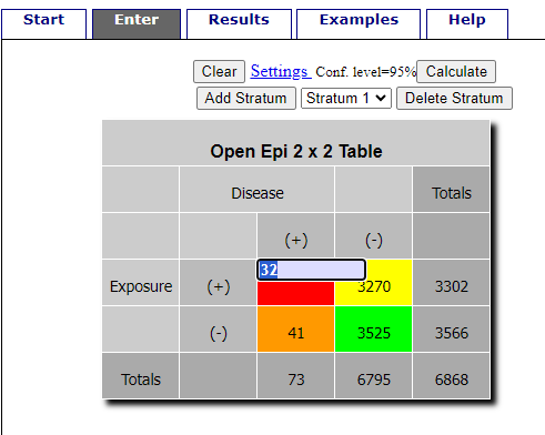
Figure 1. Data entry for 2X2 table at openepi.com.
Once the data are entered, click on the Calculate button to return a suite of results (Fig 2).
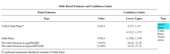
Figure 2. Results for 2X2 table at openepi.com.
Software: RcmdrPlugin.EBM
Note: Fall 2023 — I have not been able to run the EBM plugin successfully! Simply returns an error message — — on data sets which have in the past performed perfectly. Thus, until further notice, do not use the EBM plugin. Instead, use commands in the epiR package.
This isn’t the place nor can I be the author to discuss what evidence based medicine (EBM) entails (cf. Masic et al. 2008), or what its shortcomings may be (Djulbegovic and Guyatt 2017). Rcmdr has a nice plugin, based on the epiR package, that will calculate ARR, RRR and NNT as well as other statistics. The plugin is called RcmdrPlugin.EBM
install.packages("RcmdrPlugin.EBM", dependencies=TRUE)
After acquiring the package, proceed to install the plug-in. Restart Rcmdr, then select Tools and Rcmdr Plugins (Fig 3).
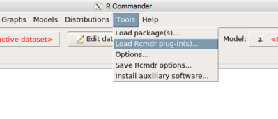
Figure 3. Rcmdr: Tools → Load Rcmdr plugins…
Find the EBM plug-in, then proceed to load the package (Fig 4).
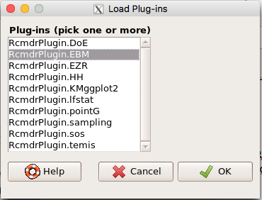
Figure 4. Rcmdr plug-ins available (after first download the files from an R mirror site).
Restart Rcmdr again and the menu “EBM” should be visible in the menu bar. We’re going to enter some data, so choose the Enter two-way table… option in the EBM plug-in (Fig 5)
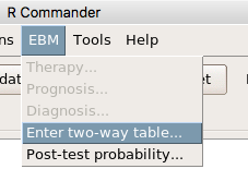
Figure 5. R Commander EBM plug-in, enter 2X2 table menus.
To review, we have the following problem, illustrated with natural numbers and probability tree (Fig 6).
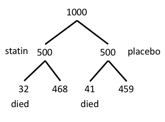
Figure 6. Illustration of probability tree for the statin problem.
Now, let’s enter the data into the EBM plugin. For the data above I entered the counts as
| Lived | Died | |
| Statin | 468 | 32 |
| Placebo | 459 | 41 |
and selected the “Therapy” medical indicator (Fig 7).
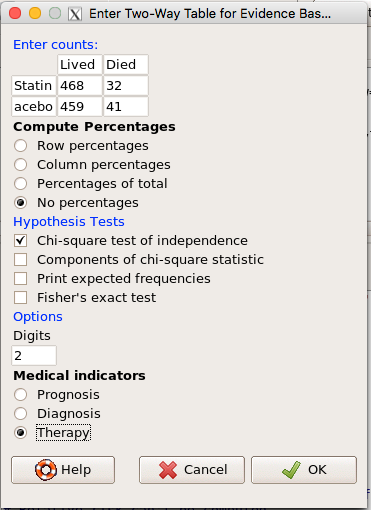
Figure 7. EBM plugin with two-way table completed for the statin problem.
The output from EBM plugin was as follows. I’ve added index numbers in brackets so that we can point to the output that is relevant for our worked example here.
(1) .Table <- matrix(c(468,32,459,41), 2, 2, byrow=TRUE, dimnames = list(c('Drug', 'Placebo'), c('Lived', 'Dead')))
(2) fncEBMCrossTab(.table=.Table, .x='', .y='', .ylab='', .xlab='', .percents='none', .chisq='1', .expected='0', .chisqComp='0', .fisher='0', .indicators='th', .decimals=2)
R output begins by repeating the commands used, here marked by lines (1) and (2). The statistics we want follow in the next several lines of output.
(3) Pearson's Chi-squared test data: .Table X-squared = 1.197, df = 1, p-value = 0.2739
(4) # Notations for calculations Event + Event -Treatment "a" "b" Control "c" "d"
(5)# Absolute risk reduction (ARR) = -1.8 (95% CI -5.02 - 1.42) %. Computed using formula: [c / (c + d)] - [a / (a + b)]
(6)# Relative risk = 1.02 (95% CI 0.98 - 1.06) %. Computed using formula: [c / (c + d)] / [a / (a + b)]
(7)# Odds ratio = 1.31 (95% CI 0.81 - 2.11). Computed using formula: (a / b) / (c / d)
(8) # Number needed to treat = -55.56 (95% CI 70.29 - Inf). Computed using formula: 1 / ARR
9)# Relative risk reduction = -1.96 (95% CI -5.57 - 1.53) %. Computed using formula: { [c / (c + d)] - [a / (a + b)] } / [c / (c + d)]
(10)# To find more about the results, and about how confidence intervals were computed, type ?epi.2by2 . The confidence limits for NNT were computed as 1/ARR confidence limits. The confidence limits for RRR were computed as 1 - RR confidence limits.
end R output
In summary, we found no difference between statin and placebo (P-value = 0.2739) and ARR of -1.8%
Questions.
Data from a case-control study on alcohol use and esophageal cancer (Tuyns et al (1977), example from Gerstman 2014). Cases were men diagnosed with esophageal cancer from a region in France. Controls were selected at random from electoral lists from the same geographical region.
| Esophageal cancer | |||
|
Alcohol grams/day |
Cases | Noncases |
Total |
| > 80 | 96 | 109 |
205 |
|
< 80 |
104 |
666 |
770 |
| Total | 200 | 775 | 975 |
- What was the null hypothesis? Be able to write the hypothesis in symbolic form and as a single sentence.
- What was the alternative hypothesis? Be able to write the hypothesis in symbolic form and as a single sentence.
- What was the observed frequency of subjects with esophageal cancer in this study? And the observed frequency of subjects without esophageal cancer?
- Estimate Relative Risk, Absolute Risk, NNT, and Odds ratio?
- Which is more appropriate, RR or OR? Justify your decision.
- The American College of Obstetricians and Gynecologists recommends that women with an average risk of breast cancer (BC) over 40 get an annual mammogram. Nationally, the sensitivity of mammography is about 68% and specificity of mammography is about 75%. Moreover, mammography involves exposure of women to radiation, which is known to cause mutations. Given that the prevalence of BC in women between 40 and 49 is about 0.1%, please evaluate the value of this recommendation by completing your analysis.
A) In this age group, how many women are expected to develop BC?
B) How many False negative would we expect?
C) How many positive mammograms are likely to be true positives? - “Less than 5% of women with screen-detectable cancers have their lives saved,” (quote from BMC Med Inform Decis Mak. 2009 Apr 2;9:18. doi: 10.1186/1472-6947-9-18): Using the information from question 5, What is the Number Needed to Treat for mammography screening?
Quiz Chapter 7.4
Epidemiology: Relative risk and absolute risk, explained
Chapter 7 contents
- Probability, Risk Analysis
- Epidemiology definitions
- Epidemiology basics
- Conditional Probability and Evidence Based Medicine
- Epidemiology: Relative risk and absolute risk, explained
- Odds ratio
- Confidence intervals
- References and suggested readings
5.1 – Experiments
How to put an experiment together
With the background behind us, we outline a designed experiment. Readers may wish to review concepts presented previously, in
- Chapter 2.4: Experimental design and rise of statistics in medical research.
- Chapter 3.4 – Estimating parameters
- Chapter 3.5 – Statistics of error
Experiments have the following elements
- Define a reference population.
- All patients with similar angina symptoms — shortness of breath, chest pain, dizziness — but who have not suffered a heart attack, or myocardial infarction (Wu et al 2017);
- All adult frogs in a pond near industrial waste runoff (eg, Sowers et al 2009).
- Define sample unit from the reference population (eg, as many patients as can be screened by the physician are recruited; all frogs visible to the biologist are captured).
- Design sampling scheme from population (eg, random sampling vs. convenience/haphazard sampling).
- Agree on the primary outcome or endpoint to be measured and whether additional secondary outcomes are to be observed and collected.
- For the patients with similar symptoms, we follow
- For the frogs, we count adults with developmental malformations.
- Separate the sample into groups so that comparisons can be made
- We may be tempted to provide the same treatment and follow the group for improvement — that is the clinically valid approach; to be an experiment, we would use random assignment of individuals to one of two groups — half will receive a placebo, half will receive a beta blocker;,
- The frog example doesn’t follow this scheme — the event has already occured, it’s an observational study.
- Devise a way to exclude or distinguish from the possible explanations, or alternative hypotheses.
- eg, for the physician, she will record how many of her patients fail to respond to treatment;
- for the biologist, noting presence or absence of parasites between the normal and abnormal frog defines the groups).
Note 1: The studies cited are examples of work done on similar problems, they are not offered to evaluate or critique any research efforts that were done or described in these reports.
The frog study, as described by me, lacks any design elements that would allow for a test of the hypothesis that industrial runoff causes developmental malformations in frogs. Students should think about how to modify this study to test the hypothesis. See quiz question.
A basic experimental design looks like this.
- One treatment, with two levels (eg, a control group and an experimental group)
- A collection of individuals recruited from a defined population, esp. by random sampling.
- Random assignment of multiple individuals to one of the two treatment levels.
- The treatments are applied to each individual in the study.
- A measure of response (the primary outcome) and additional features (secondary outcomes) are recorded for each individual.
Of course, there are other considerations, and by now, students reading this text should be able to identify what is missing from the list. (See quiz question.)
Contrast with design of observational studies
Importantly, for observational studies, no matter how sophisticated the equipment used to measure the outcome variable(s), key steps outlined above are missing. Researchers conducting observational studies do not control allocation of subjects to treatment groups (steps 4 and 3 in the two above lists, respectively). Instead, they may use case-control approaches, where individuals with (case) and without (control) the condition (eg, lung cancer) are compared with respect to some candidate risk factor (eg, smoking). Both case and control groups likely have members who smoke, but if there is an association between smoking and lung cancer, then more smokers will be in the case group compared to the control group.
A cohort study, also a form of observational study, is similar to case-control except that the outcome status is not known. A cohort study includes, in our example, smokers and non smokers who share other characteristics: age, medical history, etc. The other kind of design you will see is the cross-sectional study. Cross-sectional studies are descriptive studies, and, therefore also observational. Primary outcomes along with additional characteristics and outcomes are measured for a representative subsample, or perhaps even an entire population. Cross-sectional studies are used to absolute and relative risk rates. In ecology and evolutionary biology cross sectional studies are common, eg, comparisons of species for metabolic rate (Darveau et al 2005) or life history traits (Jennings et al 1998), and specialized statistical approaches that incorporate phylogenetic information about the species are now the hallmark of these kinds of studies.
A word on outcomes of an experiment. Experiments should be designed to address an important question. The outcomes the researcher measures should be directly related to the important question. Thus, in the design of clinical trials, researchers distinguish between primary and secondary outcomes or endpoints. In educational research the primary question is whether or not students exposed to different teaching styles (eg, lecture-style or active-learning approaches) score higher on an knowledge-content exams. The primary outcome would be the scores on the exams; many possible secondary outcomes might be collected including student’s attitudes towards the subject or perceptions on how much they have learned.
Note 3: While it’s logical to include secondary outcomes — they may offer support or complement the primary results — there needs to be caution in interpreting the test results of multiple secondary outcomes. By definition, the study is designed to test hypothesis about the primary or main outcome. While there are a number of concerns about testing secondary outcomes, from a statistical point of view, the study may lack the sample size — the power, see Chapter 11 — Power analysis — to test many additional hypotheses without the risk of increasing chance of false positives because of the multiple comparisons problem. We address this scenario in Chapter 12.1 – The need for ANOVA.
Example of an experiment.
We’ll work through a familiar example. The researcher is given the task to design a study to test the efficacy in reducing tension headache symptoms by a new pain reliever. There are many possible outcomes: blurry vision, duration, frequency, nausea, need for and response to pain medication, and level of severity (Mayo Clinic). The drug is packaged in a capsule and a placebo is designed that contains all ingredients except the new drug. Forty subjects with headaches are randomly selected from a population of headache sufferers. All forty subjects sign the consent form and agree to be part of the study. The subjects also are informed that while they are participating in the research study on a new pain reliever, each subject has a 50-50 chance of receiving a placebo and not the new drug. The researcher then randomly assigns twenty of the subjects to receive the drug treatment and twenty to receive the placebo, places either a placebo pill of the treatment pill into a numbered envelope and gives the envelopes to a research partner. The partner then gives the envelopes to the patients. Both patients and the research partner are kept ignorant of the assignment to treatment.
We can summarize this most basic experimental design in a table, Table 1.
Table 1. Simple formulation of a 2X2 experiment (aka 2×2 contingency table).
| Did the subject get better? | ||||
|---|---|---|---|---|
| Yes | No | Row totals | ||
| Subject received the treatment |
Yes | a | b | a + b |
| No | c | d | c + d | |
| Column totals | a + c | b + d | N | |
where N is the total number of subjects, a is number of subjects who DID receive the treatment AND got better, c is number of subjects who DID NOT receive the treatment, but DID get better, b is number of subjects who DID receive the treatment and DID NOT get better, and d is number of subjects who DID NOT receive the treatment and DID NOT get better.
Note 4: We owe Karl Pearson (1904) for the concepts of contingency — that membership in a (or b, c, or d for that matter) is a deviation from any chance association or independent probability (Chapter 6) — and the contingency table. Contingency is an important concept in classification and is central to machine learning in data science (Michie et al 1995). We return at some length to contingency and how to analyze contingency tables in Chapter 7 and Chapter 9.2.
And our basic expectation is that we are testing whether or not treatment levels were associated with subjects “getting better” as measured on some scale.
One possible result of the experiment, although unlikely, all of the negative outcomes are found in the group that did not receive the treatment (Table 2).
Table 2. One possible outcome of our 2X2 experiment.
| Subject improved | |||
|---|---|---|---|
| Yes | No | ||
| Subject received the treatment |
Yes | 20 | 0 |
| No | 0 | 20 | |
Results of an experiment probably won’t be as clear as in Table 2. Treatments may be effective, but not everyone benefits. Thus, results like Table 3 may be more typical.
Table 3. A more likely outcome of our 2X2 experiment.
| Subject improved | |||
|---|---|---|---|
| Yes | No | ||
| Subject received the treatment |
Yes | 7 | 13 |
| No | 2 | 18 | |
Must a control group always be included in an experiment?
To be an experiment, yes. However, it is not true that the control treatment must only be applied to separate, individual subjects. For example, a common experimental design would be repeated measures of an outcome, like behavior (eg, feeding response) before and after an intervention is applied. Thus, the individual is its own control or reference point. For example, Dohm et al (2008) measured feeding and locomotor behavior of adult toads (Rhinella marina, formerly Bufo marinus) prior to and after ozone exposure. We concluded that a single 4-h exposure to O3 depressed toad feeding behavior, but had little effect on voluntary locomotor behavior. Typically, the design randomly assigns individuals to the treatments — some individuals get the exposure first, then the control exposure second; others, again selected at random, receive the control exposure first, then the active exposure.
The within subjects design is an important method in biological research; these designs offer control for individual differences as confounding variables and require fewer participants compared to separate control group designs. This design is effective provided there is little risk of carryover effects; if the effects of a previous condition linger, then it may influence a participant’s response in subsequent conditions, confounding the results. For our study (Dohm et al 2008) we used a modified within-subjects design by employing a split plot design. We return to within-subjects designs in Chapter 14.4 – Randomized block design.
Questions
- When I updated this page in 2020, we were in our fifth month of the coronavirus pandemic of 2019-2020. Daily it seemed, we heard news about “promising coronavirus treatments,” but no study had at the time been published that would meets our considerations for a proper experiment. However, on May 1, 2020, the FDA issued an emergency use authorization for use of the antiviral drug remdesivir (Gilead), based on early results of clinical trials reported 29 April in The Lancet (Wang et al 2020). Briefly, their study included 158 treated with does of the antiviral drug and 79 provided with a placebo control. Both groups were treated otherwise the same. Improvement over 28 days was recorded: 62 improved with Placebo and 133 improved receiving dose of remdesivir.
- Using the background described on this page, list the information needed to design a proper experiment. Using your list, review the work described in The Lancet article and check for evidence that the trial meets these requirements.
- Create a 2×2 table with the described results from The Lancet article.
- Consider our hazel tea and copper solution experiment described in Chapter 3. The outcome variables (Tail length, tail percentage, Olive moment) are quantitative, not categorical. Create a table to display the experimental design.
- For the migraine example, identify elements of the design that conform to the randomized control trial design described in Chapter 2.4.
Quiz Chapter 5.1
Experiments