6.10 – t distribution
Introduction
Student’s t distribution is a sampling distribution where values are sampled from a normal distributed population, but σ the standard deviation and μ the mean of the population are not known. When sample size is large and we know σ the standard deviation, we would use the Z-score to evaluate probabilities of the sample mean. The t-distribution applies when σ is not known and sample size is small (eg, less than 30, per rule of thirty).
Note 1: According to Wikipedia and sources therein, Student was the pseudonym of William Sealy Gosset, who came up with the t-test and t-distribution.
Because of its thicker tails compared to the normal distribution, the t-distribution accounts for the uncertainty in estimating the population variability. This is important because we would require a more extreme value to be considered “statistically significant” compared to the normal distribution, making your conclusions more conservative.
Note 2: “Conservative” is a desirable characteristic in statistical inference because it means a procedure is less likely to result in a Type I error.
The equation of the t-test is

where the difference between “X bar,” the sample mean, and μ, the population mean, is divided by the standard error of the mean,  , defined in Chapter 3.2 and again in Chapter 3.3. This formulation of the t-test is called the one sample t-test (Chapter 8.5). We call the result of this calculation the test statistic for t. We evaluate how often that value or greater of a test statistic will occur by applying the t distribution function.
There are many t-distributions, actually, one for every degree of freedom. Like the normal distribution, the t distribution is always symmetrical about the mean. But it is stacked up (leptokurtic) around the middle at low degrees of freedom. As degrees of freedom increase, the t distribution spreads and becomes increasingly like the normal distribution.
Relationship between t distribution and standard normal curve.
First, here is our standard normal plot, mean = 0, standard deviation = 1 (Fig 1).
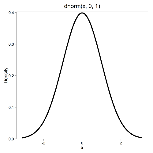
Figure 1. Density plot of standard normal distribution
Next, here’s the t-distribution for five degrees of freedom (Fig 2).
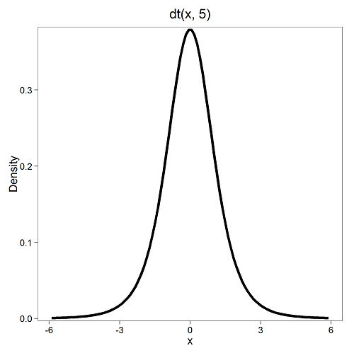
Figure 2. Density plot of t-distribution for five degrees of freedom.
Lets see what happens to the shape of the t-distribution as we increase the degrees of freedom from df = 5, 10, 20, 50, 1000, 10000 (Fig 3). The last graphic in the series is the standard normal curve again (Fig 3).
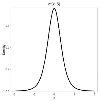
Figure 3. Animated GIF of density plot t distribution, from df = 5 to 10,000 plus standard normal curve.
By convention in the Null Hypothesis Significance Testing protocol (NHST), we compare the test statistic to a critical value. The critical value is defined as the value of the test statistic that occurs at the Type I error rate, which is typically set to 5%. We introduced logic of NHST approach in Chapter 6.9 with the chi-square distribution. Again ,this is just an introduction; we teach it now as a sort of mechanical understanding to develop. The justification for this approach to testing of statistical significance is developed in Chapter 8.
Table of Critical values of the t distribution for df 1 – 5, one tail (upper)
| df | α = 0.05 | α = 0.025 | α = 0.01 |
| 1 | 6.314 | 12.706 | 31.820 |
| 2 | 2.920 | 4.303 | 6.965 |
| 3 | 2.353 | 3.182 | 4.541 |
| 4 | 2.132 | 2.776 | 3.747 |
| 5 | 2.015 | 2.571 | 3.365 |
See Appendix 20.3 for a complete table of t-distribution.
Questions
Be able to answer these questions using the t table, Appendix 20.3, or using Rcmdr
- For probability α = 5%, what is the critical value of the t distribution (upper tail) for 1 degree of freedom? For 5 df? For 20 df? For 30 df?
- The value of the t test statistic is given as 12. With 3 degrees of freedom, what is the approximate probability of this value, or greater from the t distribution?
Quiz Chapter 6.10
t distribution
Chapter 6 contents
- Introduction
- Some preliminaries
- Ratios and proportions
- Combinations and permutations
- Types of probability
- Discrete probability distributions
- Continuous distributions
- Normal distribution and the normal deviate (Z)
- Moments
- Chi-square distribution
- t distribution
- F distribution
- References and suggested readings