12.3 – Fixed effects, random effects, and agreement
Introduction
Within discussions of one-way ANOVA models the distinction between two general classes of models needs to be made clear by the researcher. The distinction lies in how the levels of the factor are selected. If the researcher selects the levels, then the model is a Fixed Effects Model, also called a Model I ANOVA. On the other hand, if the levels of the factor were selected by random sampling from all possible levels of the factor, then the model is a Random Effects Model, also called a Model II ANOVA. This page is about such models and I’ll introduce the intraclass correlation coefficient, abbreviated as ICC, as a way to illustrate applications of Model II ANOVA.
Here’s an example to help the distinction. Consider an experiment to see if over the counter painkillers are as good as prescription pain relievers at reducing numbers of migraines over a six week period. The researcher selects Tylenol®, Advil®, Bayer® Aspirin, and Sumatriptan (Imitrex®), the latter an example of a medicine only available by prescription. This is clearly an example of fixed effects; the researcher selected the particular medicines for use.
Random effects, in contrast, implies that the researcher draws up a list of all over the counter pain relievers and draws at random three medicines; the researcher would also randomly select from a list of all available prescription medicines.
Fixed effects are probably the more common experimental approaches. To be complete, there is a third class of ANOVA called a Mixed Model or Model III ANOVA, but this type of model only applies to multidimensional ANOVA (eg, two-way ANOVA or higher), and we reserve our discussion of the Model III until we discuss multidimensional ANOVA (Table 1).
Table 1. ANOVA models
| ANOVA model | Treatments are |
| I | Fixed effects |
| II | Random effects |
| III | Mixed, both fixed & random effects |
Although the calculations for the one-way ANOVA under Model I or Model II are the same, the interpretation of the statistical significance is different between the two.
In Model I ANOVA, any statistical difference applies to the differences among the levels selected, but cannot be generalized back to the population. In contrast, statistical significance of the Factor variable in Model II ANOVA cannot be interpreted as specific differences among the levels of the treatment factor, but instead, apply to the population of levels of the factor. In short, Model I ANOVA results apply only to the study, whereas Model II ANOVA results may be interpreted as general effects, applicable to the population.
This distinction between fixed effects and random effects can be confusing, but it has broad implications for how we interpret our results in the short-term. This conceptual distinction between how the levels of the factor are selected also has general implications for our ability to acquire generalizable knowledge by meta-analysis techniques (Hunter and Schmidt 2000). Often we wish to generalize our results: we can do so only if the levels of the factor were randomly selected in the first place from all possible levels of the factor. In reality, this may not often be the case. It is not difficult to find examples in the published literature in which the experimental design is clearly fixed effects (ie, the researcher selected the treatment levels for a reason), and yet in the discussion of the statistical results, the researcher will lapse into generalizations.
Random Effects Models and agreement
Model II ANOVA is common in settings in which individuals are measured more than once. For example, in behavioral science or in sports science, subjects are typically measured for the response variable more than once over a course of several trials. Another common setting of Model II ANOVA is where more than one raters are judging an event or even a science project. In all of these cases what we are asking is about whether or not the subjects are consistent, in other words, we are asking about the precision of the instrument or measure.
In the assessment of learning by students, for example, different approaches may be tried and the instructor may wish to investigate whether the interventions can explain changes in test scores. To assess instrument validity — an item score from a grading rubric (Goertzen and Klaus 2023), tumor budding as biomarker for colorectal cancer (Bokhorst et al 2020) — agreement or concordance among two or more raters or judges (inter-rater reliability) needs to be established (same citations and references therein). For binomial data, we would be tempted to use the phi coefficient, Is it actually reliable Cohen’s kappa (two judges) or Fleiss Kappa (two or more judges) is a better tool. Phi coefficient and both assessment scores were introduced in Chapter 9.2.
For ratio scale data, agreement among scores of two or more scores from judges There is an enormous number of articles on reliability measures in the social sciences and you should be aware of a classical paper on reliability by Shrout and Fleiss (1979) (see also McGraw and Wong, 1996). Both the ICC and the Pearson product moment correlation, r, which we will introduce in Chapter 16, are measures of strength of linear association between two ratio scale variables (Jinyuan et al 2016). But ICC is more appropriate for association between repeat measures of the same thing, eg, repeat measures of running speed or agreement between judges. In contrast, the product moment correlation can be used to describe association between any two variables, eg, between repeat measures of running speed, but also between say running speed and maximum jumping height. The concept of repeatability of individual behavior or other characteristics is also a common theme in genetics and so you should not be surprised to learn that the concept actually traces to RA Fisher and his invention of ANOVA. Just as in the case of the sociology literature, there are many papers on the use and interpretation of repeatability in the evolutionary biology literature (eg, Lessels and Boag 1987; Boake 1989; Falconer and Mackay 1996; Dohm 2002; Wolak et al 2012).
Agreement and repeatability are Model II (random effects) because the subjects, items, or raters being studied are treated as a random sample from a larger population rather than specific, fixed levels of interest. In reliability studies, subjects are not chosen for their specific characteristics but as representatives of the population variability. The goal is to infer whether a measurement tool works for any future subject or rater, not just the ones tested in the study. These factors are designed to estimate variance components and generalize results beyond the specific sample used. Put another way, the goal of Model II is often to estimate how much variance is due to differences between subjects versus within subjects (repeatability), which requires treating the subject effect as random.
There are many ways to analyze these kinds of data but a good way is to treat this problem as a one-way ANOVA with Random Effects. Thus, the Random Effects model permits the partitioning of the variation in the study into two portions: the amount that is due to differences among the subjects or judges or intervention versus the amount that is due to variation within the subjects themselves. The Factor is the Subjects and the levels of the factor are how ever many subjects are measured twice or more for the response variable.
If the subjects performance is repeatable, then the Mean Square Between (Among) Subjects,  , component will be greater than the Mean Square Error component,
  , of the model. There are many measures of repeatability or reliability, but the intraclass correlation coefficient or ICC is one of the most common. The ICC may be calculated from the Mean Squares gathered from a Random Effects one-way ANOVA. ICC can take any value between zero and one.

where

and

B and W refers to the among group (between or among groups mean square) and the within group components of variation (error mean square), respectively, from the ANOVA, MS refers to the Mean Squares, and k is the number of repeat measures for each experimental unit. In this formulation k is assumed to be the same for each subject.
By example, when a collection of sprinters run a race, if they ran it again, would the outcome be the same, or at least predictable? If the race is run over and over again and the runners cross the finish lines at different times each race, then much of the variation in performance times will be due to race differences largely independent of any performance abilities of the runners themselves and the Mean Square Error term will be large and the Between subjects Mean Square will be small. In contrast, if the race order is preserved race after race: Jenny is 1st, Ellen is 2nd, Michael is third, and so on, race after race, then differences in performance are largely due to individual differences. In this case, the Between-subjects Mean Square will be large as will the ICC, whereas the Mean Square for Error will be small, and so will the ICC.
Can the intraclass correlation be negative?
In theory, no. Values for ICC range between zero and one. The familiar Pearson product moment correlation, Chapter 16, takes any value between -1 and +1. However, in practice, negative values for ICC will result if  .
.
In other words, if the within group variability is greater than the among group variability, then negative ICC are possible. The question is whether negative estimates are ever biologically relevant or, simply result of limitations of the estimation procedure. Small ICC values and few repeats increases the risk of negative ICC estimates. Thus, a negative ICC would be “simply a(n) “unfortunate” estimate (Liljequist et al 2019). However, there may be situations in which negative ICC is more than unfortunate. For example, repeatability, a quantitative genetics concept (Falconer and Mackay 1996), can be negative (Nakagawa and Schielzeth 2010).

Repeatability reflects the consistency of individual traits over time (or spatially, eg, scales on on a snake), is defined as the ratio of within individual differences and among individuals differences. Thus, within individual variance is attributed to general environmental effects,  , whereas variance among individuals is both genetic and environmental. Scenarios for which repeated measures on the same individual may occur under environmental conditions, termed specific environmental effects or
  by Falconer and Mackay (1996), that negatively affect performance are not hard to imagine — it remains to be determined how common these conditions are and whether or not estimates of repeatability are negative.
ICC Example
I extracted 15 data points from a figure about nitrogen metabolism in kidney patients following treatment with antibiotics (Figure 1, Mitch et al 1977). I used a web application called WebPlot Digitizer (https://apps.automeris.io/wpd/), but you can also accomplish this task within R via the digitize package. I was concerned about how steady my hand was using my laptop’s small touch screen, a problem that very much can be answered by thinking statistically, and taking advantage of the ICC. So, rather than taking just one estimate of each point I repeated the protocol for extracting the points from the figure three times generating a total of three points for each of the 15 data points or 45 points in all. How consistent was I?
Let’s look at the results just for three points, #1, 2, and 3.
In the R script window enter
points = c(1,2,3,1,2,3,1,2,3)
Change points to character so that the ANOVA command will treat the numbers as factor levels.
points = as.character(points)
extracts = c(2.0478, 12.2555, 16.0489, 2.0478, 11.9637, 16.0489, 2.0478, 12.2555, 16.0489)
Make a data frame, assign to an object, eg, “digitizer”
digitizer = data.frame(points, extracts)
The dataset “digitizer” should now be attached and available to you within Rcmdr. Select digitizer data set and proceed with the one-way ANOVA.
Output from oneway ANOVA command
Model.1 <- aov(extracts ~ points, data=digitizer)

 summary(Model.1)
            Df    Sum Sq   Mean Sq  F value     Pr(>F)
points       2 313.38895 156.69448 16562.49 5.9395e-12 ***
Residuals    6   0.05676   0.00946
---
Signif. codes:  0 '***' 0.001 '**' 0.01 '*' 0.05 '.' 0.1 ' ' 1

numSummary(extracts , groups = points,
+   statistics=c("mean", "sd"))
         mean           sd data:n
1  2.04780000 0.0000000000      3
2 12.15823333 0.1684708085      3
3 16.04890000 0.0000000000      3
End R output. We need to calculate the ICC

I’d say that’s pretty repeatable and highly precise measurement!
But is it accurate? You should be able to disentangle accuracy from precision based on our previous discussion (Chapter 3.5), but now in the context of a practical way to quantify precision.
ICC calculations in R
We could continue to calculate the ICC by hand, but better to have a function. Here’s a crack at the function to calculate ICC along with a 95% confidence interval.
myICC <- function(m, k, dfN, dfD) {
 testMe <- anova(m)
 MSB <- testMe$"Mean Sq"[1]
 MSE <- testMe$"Mean Sq"[2]
 varB <- MSB - MSE/k
 ICC <- varB/(varB+MSE)
 fval <- qf(c(.025), df1=dfN, df2=dfD, lower.tail=TRUE)
 CI = (k*MSE*fval)/(MSB+MSE*(k-1)*fval)
 LCIR = ICC-CI
 UCIR = ICC+CI
 myList = c(ICC, LCIR, UCIR)
 return(myList)
}
The user supplies the ANOVA model object (eg, Model.1 from our example), k, which is the number of repeats per unit, and degrees of freedom for the among groups comparison (2 in this example), and the error mean square (6 in this case). Our example, run the function
m2ICC = myICC(Model.1, 3, 2,6); m2ICC
and R returns
[1] 0.9999396 0.9999350 0.9999442
with the ICC reported first, 0.9999396, followed by the lower limit (0.9999350) and the upper limit (0.9999442) of the 95% confidence interval.
Instead of writing your own function, several R packages can calculate the intraclass correlation coefficient (ICC) and its variants. These packages include: irr, psy, psych, and rptR. For complex experiments involving multiple predictor variables, these packages are helpful for obtaining the correct ICC calculation (cf Shrout and Fleiss 1979; McGraw and Wong 1996). For the one-way ANOVA it is easier to just extract the information you need from the ANOVA table and run the calculation directly. We do so for a couple of examples.
Example: Are marathon runners consistent more consistent than my commute times?

Figure 1.Honolulu Marathon 2024 participant. Image credit: Pdubs.94, licensed under CC BY 4.0 (Creative Commons Attribution 4.0 International License), via Wikipedia.
A marathon is 26 miles, 385 yards (42.195 kilometers) long (World Athletics.org). And yet, tens of thousands of people choose to run in these events. For many, running a marathon is a one-off, the culmination of a personal fitness goal. For others, it’s a passion and a few are simply extraordinary, elite runners who can complete the courses in 2 to 3 hours (Table 3). That’s about 12.5 miles per hour. For comparison, my 20 mile commute on the H1 freeway on Oahu typically takes about 40 minutes to complete, or 27 miles per hour (Table 2, yes, I keep track of my commute times, per Galton’s famous maxim: “Whenever you can, count”).

Figure 2. View west along Interstate H-1 (Lunalilo Freeway) at 6:30AM on a weekday, Honolulu, Oahu, Hawaii. Image used with permission, credit: S. Dohm.
Table 2. A sampling of average commute speeds, miles per hour (mph), on the H1 freeway during DrD’s morning commute (distance about 19.3 miles).
| Week | Monday | Tuesday | Wednesday | Thursday | Friday |
|---|---|---|---|---|---|
| 1 | 28.5 | 23.8 | 28.5 | 30.2 | 26.9 |
| 2 | 25.8 | 22.4 | 29.3 | 26.2 | 27.7 |
| 3 | 26.2 | 22.6 | 24.9 | 24.2 | 34.3 |
| 4 | 23.3 | 26.9 | 31.3 | 26.2 | 30.2 |
Try on your own.
Calculate the ICC for my commute speeds.
Run the one-way ANOVA to get the necessary mean squares and input the values into our ICC function. We have
require(psych)
m2ICC = myICC(AnovaModel.1, 4, 4,11); m2ICC
[1] 0.7390535 0.6061784 0.8719286
Repeatability, as estimated by the ICC, was 0.74 (95% CI 0.606, 0.872), for repeat measures of commute times.
We can ask the same about marathon runners — how consistent from race to race are these runners? The following data are race times drawn from a sample of runners who completed the Honolulu Marathon in both 2016 and 2017 in 2 to 3 hours (times recorded in minutes). In other words, are elite runners consistent?
Table 3. Honolulu marathon running times (min) for eleven repeat, elite runners.
| ID | Time |
|---|---|
| P1 | 179.9 |
| P1 | 192.0 |
| P2 | 129.9 |
| P2 | 130.8 |
| P3 | 128.5 |
| P3 | 129.6 |
| P4 | 179.4 |
| P4 | 179.7 |
| P5 | 174.3 |
| P5 | 181.7 |
| P6 | 177.2 |
| P6 | 176.2 |
| P7 | 169.0 |
| P7 | 173.4 |
| P8 | 174.1 |
| P8 | 175.2 |
| P9 | 175.1 |
| P9 | 174.2 |
| P10 | 163.9 |
| P10 | 175.9 |
| P11 | 179.3 |
| P11 | 179.8 |
Stacked worksheet, P refers to person, therefore P1 is person ID 1, P2 is person ID 2, and so on.
After running a one-way ANOVA, here are results for the marathon runners
m2ICC = myICC(Model.1, 2, 10,11); m2ICC
[1] 0.9780464 0.9660059 0.9900868
Repeatability, as estimated by the ICC, was 0.98 (95% CI 0.966, 0.990), for repeat measures of marathon performance. Put more simply, knowing what a runner did in 2016 I would be able to predict their 2017 race performance with high confidence, 98%!
And now, we compare: the runners are more consistent!
Clearly this is an apples-to-oranges comparison, but it gives us a chance to think about how we might make such comparisons. The ICC will change because of differences among individuals. For example, if individuals are not variable, if everyone finishes the race at the same time, then the ICC will be low (or even zero). Because there is no variance to be attributed to individual differences, the proportion of total variance explained by those differences will be being minimal.
Visualizing repeated measures.
Waterfall plot.
If just two measures, then a profile plot will do. We introduced profile plots in the paired t-test chapter (Ch10.3). For more than two repeated measures, a line graph will do (see question 9 below). Another graphic increasingly used is the waterfall plot (waterfall chart), particularly for before and after measures or other comparisons against a baseline. For example, it’s a natural question for our eleven marathon runners — how much did they improve on the second attempt of the same course? Figure 3 shows my effort to provide a visual.
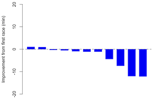
Figure 3. Simple waterfall plot of race improvement for Table 3 data. Dashed horizontal line at zero.
R code
Data wrangling: Create a new variable, eg, race21, by subtracting the first time from the second time. Multiply by -1 so that improvement (faster time in second race) is positive. Finally, apply descending sort so that improvement is on the left and increasingly poorer times are on the right.
df <- data.frame(
ID = rep(paste0("P", 1:11), each = 2),
Time = c(179.9,192.0,
129.9,130.8,
128.5,129.6,
179.4,179.7,
174.3,181.7,
177.2,176.2,
169.0,173.4,
174.1,175.2,
175.1,174.2,
163.9,175.9,
179.3,179.8)
)

# Convert to wide format
df_wide <- reshape(df, idvar = "ID", timevar = "ID",
direction = "wide")

# Extract first and second times manually
time_matrix <- matrix(df$Time, ncol = 2, byrow = TRUE)
colnames(time_matrix) <- c("Time1", "Time2")

# Calculate improvement (second - first)
base21 <- time_matrix[,2] - time_matrix[,1]

# Sort for waterfall display
base21 <- sort(base21, decreasing = TRUE)

# Waterfall plot
barplot(base21, col="blue", border="blue", space=0.5,
ylim=c(-20,20),
ylab="Improvement from first race (min)")
abline(h=0, lty=2)
Interpretation.
From the graph (Fig 3) we see that few of the racers improved their times the second time around — a few had decreased times.
Spaghetti plots.
Spaghetti plots, which display individual trajectories over time or multiple measurements, is a specialized line plot effective for visualizing the consistency of performance. The vertical thickness or spread of a single subject’s line across measurements indicates their level of repeatability. A “flat” line indicates high repeatability, while a volatile, zig-zagging line indicates low repeatability. Spaghetti plots are useful to visualize growth, decline, or stability over time for a single performance measure.
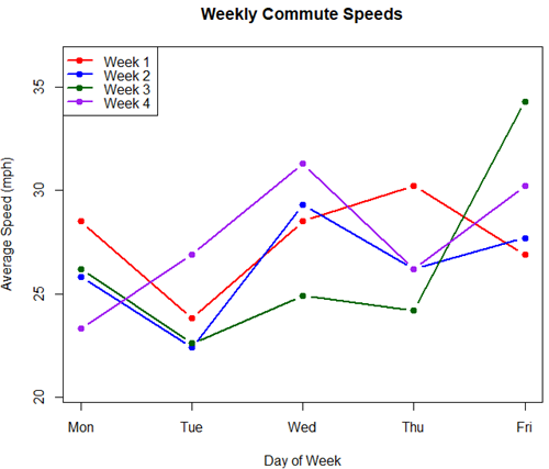
Figure 4. A spaghetti plot of average commute speeds from Table 2 data.
R code
# 1. Enter the data from Table 2.
commute <- data.frame(
Week = 1:4,
Monday = c(28.5, 25.8, 26.2, 23.3),
Tuesday = c(23.8, 22.4, 22.6, 26.9),
Wednesday = c(28.5, 29.3, 24.9, 31.3),
Thursday = c(30.2, 26.2, 24.2, 26.2),
Friday = c(26.9, 27.7, 34.3, 30.2)
)

head(commute)

# 2. Set the X-axis points
days <- 1:5
day_names <- c("Mon", "Tue", "Wed", "Thu", "Fri")

# 3. Create empty plot
# Find range of Y to ensure all data fits
ymin <- min(commute[, 2:6]) - 2
ymax <- max(commute[, 2:6]) + 2

plot(NA, xlim = c(1, 5), ylim = c(ymin, ymax),
xlab = "Day of Week", ylab = "Average Speed (mph)",
main = "Weekly Commute Speeds", xaxt = "n")

# Add X-axis labels
axis(1, at = 1:5, labels = day_names)

# 4. Add lines for each week (spaghetti)
colors <- c("red", "blue", "darkgreen", "purple")
for (i in 1:nrow(commute)) {
# Plot lines
lines(days, commute[i, 2:6], col = colors[i], lwd = 2, type = "b", pch = 19)
}

# 5. Add legend
legend("topleft", legend = paste("Week", 1:4), col = colors, lwd = 2, pch = 19)
Parallel coordinates plots.
Parallel coordinates plot allows each entity to be represented by a unique, continuous line traced across several vertical axes (each representing a different measurement or variable). High repeatability is indicated when a line remains roughly horizontal across all axes, while poor repeatability is visualized as lines that zig-zag or change direction between measurements.
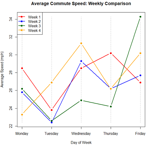
Figure 5. A parallel coordinates plot of average commute speeds from Table 2 data.
Both spaghetti plots and parallel coordinate plots can be used to visualize consistency of performance over multiple measures, but they differ significantly in their handling of data, scale, and context. Spaghetti plots are best for tracking within-subject variability over time, but quickly become a mess — like pasta tossed and sticking to a wall — when subject count increases. Parallel coordinate plots are a multivariate generalization — each line represents an individual’s profile across different tests, eg, accuracy, speed, VO2max.
R code.
# 1. Create the data frame
# see above

# 2. Extract only the numerical commute data for plotting
commute_data <- commute[, 2:6]

# 3. Setup the plot area
# Define range for y-axis
y_range <- range(commute_data)
# Define number of days (5)
num_days <- ncol(commute_data)

# Create empty plot
plot(NA, xlim = c(1, num_days), ylim = y_range,
xaxt = "n", xlab = "Day of Week", ylab = "Average Speed (mph)",
main = "Average Commute Speed: Weekly Comparison")

# Add x-axis labels
axis(1, at = 1:num_days, labels = colnames(commute_data))

# 4. Draw vertical lines for each day
for (i in 1:num_days) {
lines(c(i, i), y_range, col = "grey", lty = 2)
}

# 5. Add lines for each week (repeated measures)
colors <- c("red", "blue", "darkgreen", "orange")
for (i in 1:nrow(commute_data)) {
lines(1:num_days, commute_data[i, ], col = colors[i], lwd = 2, type = "b", pch = 19)
}

# 6. Add legend
legend("topleft", legend = paste("Week", commute$Week), col = colors, lwd = 2, pch = 19)
Heat map.
Heat map quickly identify patterns, such as an individual’s performance improving, degrading, or remaining stable over time. For example, uniform, solid colors across rows (individuals) or columns (time/trials) indicate high consistency, while varied colors indicate poor repeatability.
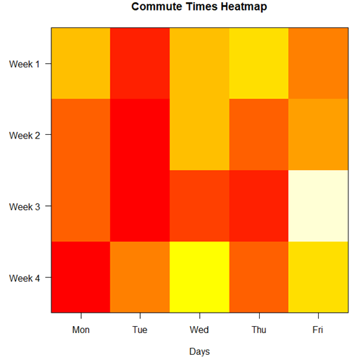
Figure 6. A heat map of the commute speeds data set.
R code.
# 1. Create the data
# Week is excluded from matrix to only include numerical commute times
commute_data <- matrix(c(
28.5, 23.8, 28.5, 30.2, 26.9,
25.8, 22.4, 29.3, 26.2, 27.7,
26.2, 22.6, 24.9, 24.2, 34.3,
23.3, 26.9, 31.3, 26.2, 30.2
), nrow = 4, byrow = TRUE)

# 2. Add row and column names
rownames(commute_data) <- c("Week 1", "Week 2", "Week 3", "Week 4")
colnames(commute_data) <- c("Mon", "Tue", "Wed", "Thu", "Fri")

# 3. Create the heatmap
# Use t() to transpose so weeks are rows and days are columns
# Use rev() on rows to have Week 1 at the top
image_data <- t(apply(commute_data, 2, rev))

# Set up the plotting area (margins for labels)
par(mar = c(5, 6, 4, 2))

# Plot the matrix
# Option 1
image(1:nrow(image_data), 1:ncol(image_data), image_data,
col = heat.colors(12),
axes = FALSE, xlab = "Days", ylab = "",
main = "Commute Times Heatmap")

# Add axes labels
axis(1, at = 1:5, labels = colnames(commute_data))
axis(2, at = 1:4, labels = rev(rownames(commute_data)), las = 1)
box()
Interpretation.
The graphs (Fig 4 – 6) show a lack of trends in consistency of drive speeds. The heat map suggests more consistency on Monday — low speeds (Fig 4 & Fig 5), but that’s a stretch.
An example for you to work, from our Measurement Day
If you recall, we had you calculate length and width measures on shells from samples of gastropod and bivalve species. In the table are repeated measures of shell length, by caliper in mm, for a sample of Conus shells (Fig 7 and Table 4).
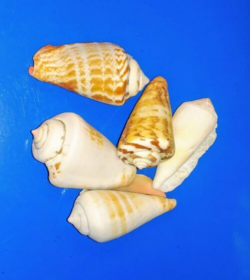
Figure 7. Conus shells, image by M. Dohm.
Repeated measures of the same 12 Conus shells.
Table 4. Unstacked dataset of repeated length measures on 12 shells
| Sample | Measure1 | Measure2 | Measure3 |
|---|---|---|---|
| 1 | 45.74 | 46.44 | 46.79 |
| 2 | 48.79 | 49.41 | 49.67 |
| 3 | 52.79 | 53.45 | 53.36 |
| 4 | 52.74 | 53.14 | 53.14 |
| 5 | 53.25 | 53.45 | 53.15 |
| 6 | 53.25 | 53.64 | 53.65 |
| 7 | 31.18 | 31.59 | 31.44 |
| 8 | 40.73 | 41.03 | 41.11 |
| 9 | 43.18 | 43.23 | 43.2 |
| 10 | 47.1 | 47.64 | 47.64 |
| 11 | 49.53 | 50.32 | 50.24 |
| 12 | 53.96 | 54.5 | 54.56 |
Maximum length from from anterior end to apex with calipers. Repeated measures were conducted blind to shell id, sampling was random over three separate time periods.
Questions
- Consider data in Table 2, Table 3, and Table 4. True or False: The arithmetic mean is an appropriate measure of central tendency. Explain your answer.
- Enter the shell data into R; Best to copy and stack the data in your spreadsheet, then import into R or R Commander. Once imported, don’t forget to change Sample to character, otherwise R will treat Sample as ratio scale data type. Run your one-way ANOVA and calculate the intraclass correlation (ICC) for the dataset. Is the shell length measure repeatable?
- The marathon results in Table 2 are paired data, results of two races run by the same individuals. Make a profile plot for the data (see Ch10.3 for help).
- A profile plot is used to show paired data; for two or more repeat measures, use a line graph instead.
A. Produce a line graph for data in Table 4. The line graph is an option in R Commander (Rcmdr: Graphs Line graph…), and can be generated with the following simple R code:
lineplot(Sample, Measure1, Measure2, Measure3)
B. What trends, if any, do you see? Report your observations.
C. Make another line plot for data in Table 2. Report any trend and include your observations.
Quiz Chapter 12.3
Fixed effects, random effects, and agreement
Chapter 12 contents
- Introduction
- The need for ANOVA
- One way ANOVA
- Fixed effects, random effects, and agreement
- ANOVA from “sufficient statistics”
- Effect size for ANOVA
- ANOVA posthoc tests
- Many tests one model
- References and suggested readings