18.5 – Selecting the best model
Introduction
This is a long entry in our textbook, many topics to cover. We discuss aspects of model fitting, from why model fitting is done to how to do it and what statistics are available to help us decide on the best model. Model selection very much depends on what the intent of the study is. For example, if the purpose of model building is to provide the best description of the data, then in general one should prefer the full (also called the saturated) model. On the other hand, if the purpose of model building is to make a predictive statistical model, then a reduced model may prove to be a better choice. The text here deals mostly with the later context of model selection, finding a justified reduced model.
From Full model to best Subset model
Model building is an essential part of being a scientist. As scientists, we seek models that explain as much of the variability about a phenomenon as possible, but yet remain simple enough to be of practical use.
Having just completed the introduction to multiple regression, we now move to the idea of how to pick best models.
We distinguish between a full model, which includes as many variables (predictors, factors) as the regression function can work with, returning interpretable, if not always statistically significant output, and a saturated model.
The saturated model is the one that includes all possible predictors, factors, interactions in your experiment. In well-behaved data sets, the full model and the saturated model will be the same model. However, they need not be the same model. For example, if two predictor variables are highly collinear, then you may return an error in regression fitting.
For those of you working with meta-analysis problems, you are unlikely to be able to run a saturated model because some level of a key factor are not available in all or at least most of the papers. Thus, in order to get the model to run, you start dropping factors, or you start nesting factors. If you were unable to get more things in the model, then this is your “full” model. Technically we wouldn’t call it saturated because there were other factors, they just didn’t have enough data to work with or they were essentially the same as something else in the model.
Identify the model that does run to completion as your full model and proceed to assess model fit criteria for that model, and all reduced models thereafter.
In R (Rcmdr) you know you have found the full model when the output lacks “NA” strings (missing values) in the output. Use the full model to report the values for each coefficient, i.e., conducting the inferential statistics.
Get the estimates directly from the output from running the regression function. You can tell if the effect is positive (look at the estimate for sample — it is positive) so you can say — more samples, greater likelihood to see more cases of cancer.
Remember, the experimental units are the papers themselves, so studies with larger numbers of subjects are going to find more cases of diabetes. We would worry big time with your project if we did not see statistically significant and positive for sample size.
Example: A multiple linear model
For illustration, here’s an example output following a run with the linear model function on a portion of the Kaggle Cardiovascular disease data set.
Note: For my training data set I simply took the first 100 rows — from the 70,000 rows! in the dataset. A more proper approach would include use of stratified random sampling, for example, by gender, alcohol use, and other categorical classifications.
The variables (and data types) were
SBP = systolic blood pressure (from ap_hi)
age.years = Independent variable, ratio scale (calculated from age in days)
BMI = Dependent variable, ratio scale (calculated from height and weight variables)
active = Independent variable, physical activity, binomial
alcohol = Independent variable, alcohol use, binomial
cholesterol = Independent variable, cholesterol levels (scored 1 = “normal,” 2 = “above normal, and 3 = “well above normal”)
gender = Independent variable, binomial
glucose = Independent variable, glucose levels (scored 1 = “normal,” 2 = “above normal, and 3 = “well above normal”)
smoke = Independent variable, binomial
R output
Call:
lm(formula = SBP ~ BMI + gender + age.years + active + alcohol +
cholesterol + gluc + smoke, data = kaggle.train)

Residuals:
Min 1Q Median 3Q Max
-33.359 -9.701 -1.065 8.703 45.242

Coefficients:
             Estimate Std. Error t value   Pr(>|t|)
(Intercept)   76.7664    14.9311   5.141  0.00000155 ***
BMI            0.8395     0.2933   2.862  0.00522 **
gender        -2.0744     1.6102  -1.288  0.20092
age.years      0.2742     0.2403   1.141  0.25672
active         7.1411     3.4934   2.044  0.04383 *
alcohol       -7.9272     9.1854  -0.863  0.39039
cholesterol    7.4539     2.3200   3.213  0.00182 **
gluc          -1.2701     2.9533  -0.430  0.66817
smoke         11.4132     6.7015   1.703  0.09197 .
---
Signif. codes: 0 '***' 0.001 '**' 0.01 '*' 0.05 '.' 0.1 ' ' 1

Residual standard error: 14.96 on 91 degrees of freedom
Multiple R-squared: 0.2839, Adjusted R-squared: 0.221
F-statistic: 4.51 on 8 and 91 DF, p-value: 0.0001214
Question. Write out the equation in symbol form.
We see from the modest R2 (adjusted) that the model explains little variation in systolic blood pressure; only BMI, physical activity (yes, no), and serum cholesterol levels, were statistically significant at 5% level. Smoker (yes, no) approached significance (p-value = 0.092), but I wouldn’t go on and on about positive or negative coefficients and effects.
Note: For my training data set I simply took the first 100 rows — from the 70,000 rows! in the dataset. A more proper approach would include use of stratified random sampling, for example, by gender, alcohol use, and other categorical classifications.
We report the value (I would round to 7.5) for cholesterol on SBP (Table 1), and note that those who had elevated serum cholesterol levels tended to have higher systolic blood pressure (e.g., the sign of the coefficient — and I related the coefficient back to the most important thing about your study — the biological interpretation). Repeat the same for the other significant coefficients.
Now’s a good time to be clear about HOW you report statistical results. DO NOT SIMPLY COPY AND PASTE EVERYTHING into your report. Now, for the estimates above, you would report everything, but not all of the figures. Here’s how the output should be reported in your Project paper.
Table 1. Coefficients from full model.
term     Coefficient Error  P-value*
Intercept       76.8  14.93 < 0.00001
BMI              0.8   0.29   0.00522
gender          -2.1   1.61   0.20092
age.years        0.3   0.24   0.25672
active           7.1   3.49   0.04383
alcohol         -7.9   9.19   0.39039
cholesterol      7.5   2.32   0.00182
gluc            -1.3   2.95   0.66817
smoke           11.4   6.70   0.09197
* t-test
Looks better, doesn’t it?
Note: Obviously, don’t round for calculations!
Once you have the full model, we should run simple diagnostics on the regression fit to the data (VIF, Cook’s Distance, basic diagnostic plots), then proceed to use this model for the inferential statistics.
> vif(model.1)
BMI gender age.years active alcohol cholesterol gluc smoke
1.112549 1.091154 1.081641 1.048519 1.096382 1.178635 1.168442 1.131081
No VIF was greater than 2, suggesting little multicollinearity among the predictor variables.
> cooks.distance(model.1)[which.max(cooks.distance(model.1))]
60
0.355763
This person had high SBP (180), was a smoker, but active and normal BMI.
Use the significance tests of each parameter in the model from the corresponding ANOVA table. Now, where is the ANOVA table? Remember, right after running the linear regression,
Rcmdr: Models → Hypothesis testing → ANOVA tables
Accept the default (partial marginality), and, Boom! … the ANOVA table you should be familiar with.
From the ANOVA table you will tell me whether a Factor is significant or not. You report the ANOVA table in your paper. You describe it.
Now, the next step is to decide what is the best model. It then guides you to the next step which is to decide whether a better model (fewer parameters, Occam’s razor) can be found. Identify the parameter from the ANOVA table with the highest P-value and remove it from the model when you run the regression again. Repeat the steps above, return the ANOVA table, checking the estimates and P-values, until you have a model with only statistically significant parameters.
Find the best model
We may be tempted to run the linear model again, but with non-significant predictors excluded. For example, re-run the model on SBP but with just BMI, active, cholesterol and excluding smoke.
We can calculate the AIC, Akaike Information Criterion, the lower value is considered the better model.
AIC(model.1)
[1] 835.4938
AIC(model.2)
[1] 834.0782
The full model had eight predictor variables, excluding the intercept, whereas the reduced model had just three predictor variables, again, not including the intercept. Unsurprisingly, the reduced model is better. But now, a stronger test — what about smoking, where the p-value approached 5%? We ran the linear model (model.3).
> AIC(model.3)
[1] 831.9495
We can use an anova test or the likelihood ratio test to compare the models. The anova test, the models must be nested.
stats::anova(model.2, model.3)
Analysis of Variance Table

Model 1: SBP ~ BMI + active + cholesterol
Model 2: SBP ~ BMI + active + cholesterol + smoke
  Res.Df   RSS Df Sum of Sq      F   Pr(>F)
1     96 22205
2     95 21307  1     898.1 4.0043 0.04824 *
---
Signif. codes: 0 '***' 0.001 '**' 0.01 '*' 0.05 '.' 0.1 ' ' 1
and
lmtest::lrtest((model.2,model.3)
Likelihood ratio test

Model 1: SBP ~ BMI + active + cholesterol
Model 2: SBP ~ BMI + active + cholesterol + smoke
 #Df  LogLik Df  Chisq Pr(>Chisq)
1  5 -412.04
2  6 -409.97  1 4.1286 0.04216 *
---
Signif. codes: 0 '***' 0.001 '**' 0.01 '*' 0.05 '.' 0.1 ' ' 1
Both tests tell us the same thing — our model with four predictors, including smoking, is better.
2 December 2024 — Past this point, edits pending
But first, I want to take up an important point about your models that you may not have had a chance to think about. The order of entry of parameters in your model can effect the significance and value of the estimates themselves. The order of parameter model entry above can be read top to bottom. Age was first, followed in sequence by CalsPDay, CholPDay, and so on. By convention, enter the covariates first (the ratio-scale predictors), that’s what I did above.
Here’s the output from a model in which I used a different order of parameters.
Anova(LinearModel.2, type="II")
Anova Table (Type II tests)

Response: BMI
              Sum Sq    Df    F value     Pr(>F)
Sex             1.52     1     0.0478    0.82764
Smoke           8.84     1     0.2782    0.59964
Age             0.62     1     0.0196    0.88918
CalsPDay       10.79     1     0.3394    0.56215
CholPDay       92.37     1     2.9065    0.09286 .
Sex:Smoke       3.35     1     0.1055    0.74631
Residuals    2129.34    67
The output is the same!!! So why did I give you a warning about parameter order? Run the ANOVA table summary command again, but this time select Type III type of test, i.e., ignore marginality
> Anova(LinearModel.2, type="III")
Anova Table (Type III tests)

Response: BMI
               Sum Sq    Df    F value       Pr(>F)
(Intercept)   1544.34     1    48.5929   1.708e-09 ***
Sex              4.69     1     0.1475     0.70214
Smoke           11.82     1     0.3720     0.54400
Age              0.62     1     0.0196     0.88918
CalsPDay        10.79     1     0.3394     0.56215
CholPDay        92.37     1     2.9065     0.09286 .
Sex:Smoke        3.35     1     0.1055     0.74631
Residuals     2129.34    67
The output has changed — and in fact it now reports the significance test of the intercept. This output is the same as the output from the linear model. Try again, this time selecting Type I, sequential
> anova(LinearModel.2)
Analysis of Variance Table

Response: BMI
           Df   Sum Sq    Mean Sq  F value    Pr(>F)
Sex         1     0.68      0.681   0.0214   0.88402
Smoke       1     2.82      2.816   0.0886   0.76690
Age         1     3.44      3.436   0.1081   0.74333
CalsPDay    1     2.27      2.272   0.0715   0.78998
CholPDay    1    96.30     96.299   3.0301   0.08633
Sex:Smoke   1     3.35      3.354   0.1055   0.74631
Residuals  67  2129.34     31.781
Here, we see the effect of order. So, as we are working to learn all of the issues of statistics and in particular mode fitting, I have purposefully restricted you to Type II analyses — obeying marginality correctly handles most issues about order of entry.
Easy there…. Take a deep breath, and guess what? Your best model needs to have significant parameters in it, right? Your best fit model then is Model 5. And that model will be your candidate for best fit as we proceed to complete our model building.
![]()
Now we proceed to gain some support evidence for our candidate best model. We are going to use an information criterion approach.
Use a fit criterion for determining model fit
To help us evaluate evidence in favor of one model over another there are a number of statistics one may calculate to provide a single number for each model for comparison purposes. The criteria model evaluators available to us include Mallow’s Cp, adjusted R2, Akaike Information Criterion (AIC) or the Bayesian Information Criterion (BIC) to select best model.
We already introduced the coefficient of determination R2 as a measure of fit – in general we favor models with larger values of R2. However, values of R2 will always be larger for models with more parameters. Thus, the other evaluators attempt to adjust for the parameters in the model and how they contribute to increased model fit. For illustrative purposes we will use Mallow’s Cp. The equation for Mallow’s Cp in linear regression is
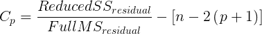
where p is the number of parameters in the model. Mallow’s Cp is thus equal to the number of parameters in the model plus an additional amount due to lack of fit of the model (i.e., large residuals). All else being equal we favor the model in which the Cp is close to the number of parameters in the model.
In Rcmdr, select Models → Subset model selection … (Fig. 1)
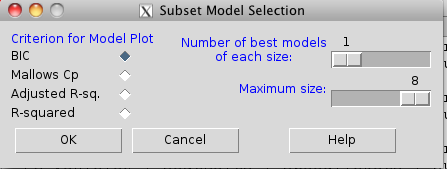
Figure 1. Rcmdr popup menu, Subset model selection…
From the menu, select the criterion and how many models to return. The function returns a graph that can be used to interpret which model is best given the selection criterion used. Below is an example (although for a different data set!) for Mallow’s Cp (Fig. 2).
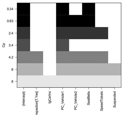
Figure 2. Mallow’s Cp plot
Lets break down the plot. First define the axes. The vertical axis is the range of values for the Cp calculated for each model. The horizontal axis is categorical and reads from left to right: Intercept, Inspection[T.Yes], etc., up to Suspended. Looking into the graph itself we see horizontal bars — the extent of shading indicates which model corresponds to the Cp value. For example, the lowest bar which is associated with the Cp value of 8 extends all the way to the right of the graph. This says that the model evaluated included all of the variables and therefore was the saturated or full model. The next bar from the bottom of the graph is missing only one block (lgCarIns), which tells us the Cp value 6 corresponds to a reduced model, and so forth.
Cross-validation
Once you have identified your Best Fit model, then, your proceed to run the diagnostics plots. For the rest of the discussion we return to our first example.
Rcmdr: Models → Graphs → Basic diagnostic plots.
We’ll just concern ourselves with the first row of plots (Fig. 3).
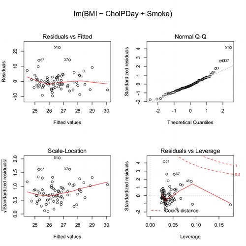
Figure 3. Diagnostic plots
The left one shows the residuals versus the predicted values — if you see a trend here, the assumption of linearity has been violated. The second plot is a test of the assumption of normality of the residuals. Interpret them (residuals OK, Residuals normally distributed? Yes/ No), and you’re done. Here, I would say I see no real trend in the residuals vs fitted plot, so assumption of linear fit is OK. For normality, there is a tailing off at the larger values of residuals, which might be of some concern (and I would start thinking about possible leverage problems), but nothing dramatic. I would conclude that our Model 6 is a good fitting model and one that could be used to make predictions.
Now, if you think a moment, you should identify a logical problem. We used the same data to “check” the model fit as we did to make the model in the first place. In particular if the model is intended to make predictions it would be advisable to check the performance of the model (e.g., does it make reasonable predictions?) by supplying new data, data not used to construct the model, into the model. If new data are not available, one acceptable practice is to divide the full data set into at least two subsets, one used to develop the model (sometimes called the calibration or training dataset) and the other used to test the model. The benefits of cross-validation include testing for influence points, over fitting of model parameters, and a reality check on the predictions generated from the model.
A note on best practices
In the 1980s, researchers often “removed” the effect of a covariate by first fitting a regression and then saving the residuals to use in separate analyses, such as t-tests, ANOVAs, or variance component estimates (eg, Dohm et al 2001). For example, in a study of plant growth, scientists might regress final plant height on initial size to remove the effect of size, then compare the residuals between fertilizer groups. While this approach adjusts for the covariate, it is problematic because residuals are not raw data: they are correlated, have constrained sums, and underestimate uncertainty. This can distort group differences, especially if the covariate distributions differ among groups, and it ignores the variability introduced by the first regression. This approach was common in ecology, evolutionary biology, physiology, and psychology before modern mixed modeling and generalized regression workflows became standard.
Modern best practices instead recommend fitting a single unified model that includes both the covariate and the grouping variable directly. Using the same plant growth example, a linear model such as  estimates the effect of fertilizer while properly accounting for initial plant size. This approach provides valid standard errors, allows correct inference about group differences, and can accommodate interactions (eg, if the relationship between
  and
and  differs by group) or hierarchical data structures using mixed-effects models. Additionally, modern workflows include diagnostics such as residual plots, Cook’s Distance, and variance inflation factors to check model assumptions and influential points. Use mixed models when data are hierarchical or repeated data. Random effects handle variation among groups, individuals, years, etc., in a single coherent model. When covariates need to be “controlled for,” we use partial regression. This happens inside the model, not by subtracting covariate effects first. By analyzing all relevant predictors in a single model, researchers obtain more accurate estimates, properly reflect uncertainty, and avoid the statistical pitfalls of the old residual-based two-stage approach.
Thus, there are several statistical reasons the older approach fails under modern scrutiny. First, Residuals are not independent observations. Residuals are model-dependent quantities, not raw data. Once you fit a regression, the residuals are correlated with each other, constrained to sum to zero, and, likely heteroscedastic if the model was imperfect. Using them in a new test violates standard assumptions of the second test.
Second, you underestimate uncertainty. If you perform tests on residuals, the standard errors do not include uncertainty from the first regression, which may lead to inflated Type I error and an overly confident “adjusted” group comparisons.
Third, the old approach creates a “two-stage model” that breaks the likelihood framework. A two-stage analysis discards the correct joint likelihood and therefore produces biases p-values, and interferes with valid confidence intervals or predictions.
Under the modern one-stage models include ML/REML, generalized estimating equations, and fully integrated Bayesian models, which keeps the model coherent. Use of mixed models make residualization unnecessary. In studies with repeated measures, blocks, sites, subjects, or years, the old approach cannot partition sources of variation correctly.
In short, the advantages of the one-stage approach is that resulting models have valid uncertainty, correct group comparisons, better handling of interactions and hierarchy, full likelihood-based inference. They fit a single unified regression or mixed-effects model with all relevant predictors, examine diagnostics, and make inferences directly. This is one more benefit of the increased power and availability of more powerful computers and more complete development of mixed methods modeling.
Questions
- Write up three learning outcomes for this page. Hint: Point your favorite generative AI to this page and ask for help.
Quiz Chapter 18.5
Selecting the best regression model