2.3 – A brief history of (bio)statistics

Foundations of biostatistics: key definitions

.

Before discussing history and landmark moments in biostatistics, let’s start with basic definitions.

Bioinformatics is loosely defined as a discipline of biology primarily concerned with work involving large data sets (e.g., databases), but a bioinformatician would not primarily be a statistician necessarily. Rather, a bioinformatician in addition to foundation in statistical and mathematical training would likely be fluent in at least one programming language and confident in use and design of databases.

Biostatistics, or biometry, then, refers to use of statistics in biology. Biostatistics encompasses application of statistical approaches to design, analyze, and interpret biological data collected through observation of use of experimentation. In turn, there are many broad disciplines or fields of specialty that trained biostatisticians may work.

Chance, the likelihood that a particular event will occur.

Data scientist, a very general label, is a person likely to work on “big data.” Big data may be loosely and inconsistently identified as access to large detailed and unstructured data sets such as visits and behavior within websites of tens of millions of Internet “hits” to a website like Amazon® or Google®. The data scientist would then be involved in extracting meaning from volumes of this data in a process called data mining. In the context of biology web sites like ALFRED at Yale University which houses allele frequency information collected on human populations, the 1000 genome project, or any of the databases accessible at National Center for Biotechnology Information would constitute sources of big data for biological researchers.

Epidemiology refers to the statistics of patterns of and risk of disease in populations, particularly of humans and thus, an epidemiologist would also be considered to be a biostatistician. The statistics of epidemiology include all of the materials we will cover in this course, but perhaps if any particular analytical approach characterizes epidemiology, it would be survival analysis (review in Clark et al 2003) — in competition with compartment models to predict spread of communicable disease in populations (Brauer 2017).

Event, an outcome to which a probability is assigned.

Likelihood, the probable chance of occurrence of an event that has already occurred. Likelihood assesses how well a particular model or set of parameters explains observed data.

Probability, the chance that an event will occur in the future, given a known model or set of parameters.

Random or random chance. This is a good place to share a warning about vocabulary; statistics, like most of science, uses familiar words, but with refined and sometimes different meanings than our everyday usage. Consider our everyday use of random: “without definite aim, direction, rule, or method – subjects chosen at random” (Merriam-Webster online dictionary). In statistics, however, random refers to “an assignment of a numerical value to each possible outcome of an event” (Wikipedia, Eagle 2021). Thus, in statistics, random dictates a method of determining how likely a subject is to be included: If represents the size of the population, then random sampling implies that each individual had chance of being selected. Thus, if , then each individual has a 1% () chance of selection. This is quite different from Merriam-Webster’s definition, in which no method is assumed. To a statistician, then, random as used in everyday conversation would imply haphazard sampling or convenience sampling from a population.

Statistics may be defined as the science of collecting, organizing, and interpreting data. Statistics is a branch of applied mathematics. Note that the word statistic is also used, but refers to a calculated quantity like the mean or standard deviation. A little confusing, but the context in which statistics or statistic is appropriate is usually not a major issue.

From dice games to data science: A brief history of statistics

.

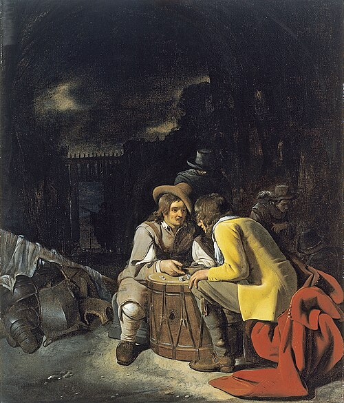
Figure 1. Soldiers playing dice, painting by Michiel Sweerts (1618–1664). Public domain image, https://commons.wikimedia.org/

The concepts of chance and probability, so crucial to statistical reasoning — because it allows us to interpret data when outcomes are inconsistent — were realized rather late in the history of mathematics. While people have been writing about applied and theoretical math for thousands of years, probability as a topic of interest by (Western) scholars seems to date only back to the late 17th century, beginning with letters written between Pierre de Fermat (1601-1665) and Blaise Pascal (1623 – 1662) and the substantial work on probability by Pierre-Simon Laplace (1749-1827). Often, research on probability developed under the watchful eyes of rich patrons more interested in gaming (sensu Fig 1), than to scientific applications. Work on permutations and combinations, essential for an understanding of probability, trace to India prior to Pascal’s work (Raju 2011).

The history of statistics goes back further if you allow for the dual use of the term statistics, both as a descriptor of the act of collecting data and as a systematic approach to the analysis of data. Prior to the 1700s, statistics was used in the sense of collection of data for use by the governments. It is not until the latter part of the 19th century that we see scholarship on statistical analytical techniques. Many of the statistical approaches we teach and use today were developed in the decades between 1880s and the 1930s. Work by Francis Galton (1822-1911), Karl Pearson (1857-1936), R. A. Fisher (1890-1962), Sewall Wright (1889-1988), Jerzy Neyman (1894-1981), Egon Pearson (1895-1980, Karl Pearson’s son), George E. P. Box (1919-2013) remains highly influential today.

Development of randomized controlled (clinical) trials, RCT, the “gold standard,” by the 1950s provides the strongest study design to evaluate the effectiveness of clinical or other kinds of interventions. The general features of RCT are (1) comparison among groups, with at least one control group, (2) randomization, and (3) blinding, where treatment options are concealed from the subjects (single-blind) and from those charged to assess the outcomes (double-blind). Sir Austin Bradford Hill (1887-1991) is generally credited with developing the RCT (Collier 2009, Matthews 2016), but we owe RA Fisher for randomization in experimental design. Hill (1965) is also known for Hill’s criteria of causality — nine principles that can be used to establish causal relationship between epidemiological (observational) evidence and disease. Chief among these nine principles are strength of the association (effect size) and consistent association (reproducibility), elements we return to often in our introduction to biostatistics.  

Since the 1950s, there has been an explosion of developments in statistics, particularly as related to power of computer. These include use of resampling, simulation, and Monte Carlo methods (Harris 2010). Resampling — the creation of new samples based on a set of observed data — is a key innovation in statistics. Its use led to a number of innovative ways to estimate the precision of an estimate (see Chapter 3.4 and Chapter 19). Monte Carlo methods, or MCM, which involves resampling from a probability distribution, is used to repeat (simulate) an experiment over and over again (Kroese et al 2014). Computers have so influenced statistics that some now define statistics as “…the study of algorithms for data analysis” (p. 175, Beran 2003). So much so, the role of computers and coding to process and model data, we now have the discipline of Data Science. For more on the history of statistics, see Anderson (1992), Fienberg (1992), and Freedman 1999; for excellent, conversational books read Salsburg (2002) and McGrayne (2011). For influential women in early development of statisticians, see Anderson (1992).

Numbers and prejudice: A hidden history of statistics

.

Many statistical methods in use today, including regression and analysis of variance methods, can trace their origins to the late 1800’s and early 1900’s (Kevles 1998). Many of these early statisticians developed statistical methods to, at least in part, further their interests in understanding differences between racial groups of humans. Sir Francis Galton, who developed regression and correlation concepts (the details and extensions of which were the works of Karl Pearson), coined the term Eugenics, the “science” of improving humans through selective breeding. In an editorial, the journal Nature recently published an apology for it’s complicity providing “a platform to [eugenicists] views” (p. 875, Nature 2022). Sir R. A. Fisher is rightfully remembered as the inventor of analysis of variance and maximum likelihood techniques (Rao 1992; Bodmer et al 2021), and perhaps more important, developed the concepts of sampling from populations, degrees of freedom, among other contributions. However, he was an active promoter of eugenics (Bodmer et al 2021), and an award given by The Society for the Study of Evolution in his honor, the R.A. Fisher Prize, was renamed in 2020.

Eugenics is still with us (see Legacies of Eugenics: An Introduction Los Angeles Review of Books; Veit et al 2021), but the era of “Three generations of imbeciles are enough” (Buck v. Bell), and the forced sterilization eugenic programs of the Nazi (Kelves 1999), were thoroughly discredited on scientific grounds many times (click here for Eugenics Archive website). Do keep in mind that the times were different, and elements of eugenics thinking remains with us (cf. discussion in Veil et al 2021 and references therein), it is interesting nevertheless to learn about the murky history of statistics and the objectives of some of the very bright people responsible for many of the statistical analyses we use today (see Stephan J. Gould’s “The Mismeasure of Man“). Several books tackle aspects of scientific racism, including 2017 Is science racist? by Jonathan Marks and 2019 Superior: The return of of race science, by Angela Saini and a host of articles and books listed at Wikipedia.

Keep in mind also that statisticians were instrumental in showing why Eugenics was unscientific, at best. See 2021 review by Rebecca Sear, Demography and the rise, apparent fall, and resurgence of eugenics, in Population studies: A journal of demography. While the algorithms of statistics are unbiased, clearly, humans, and the interpretations of data may be biased. Statistical reasoning absolutely requires considering sources of bias and their impacts on our conclusions.

Landmark epidemiology studies

.

John Snow (1813-1858) is credited by some as the “Father of Epidemiology”(Ramsay 2006). During a London outbreak — the sudden increase of disease events — of cholera in 1854, Snow conducted work to establish cholera mortality with source and quality of drinking water. At the time, the prevailing explanation for cholera was that it was an airborne infection. Snow’s map of cholera mortality in the Golden Square district of London in relation to a water pump on Broad Street is shown in Fig 2, Snow’s theory of contaminated water was not accepted as an explanation for cholera until after his death.

Original map by John Snow showing the clusters of cholera cases in the London epidemic of 1854, drawn and lithographed by Charles Cheffins.

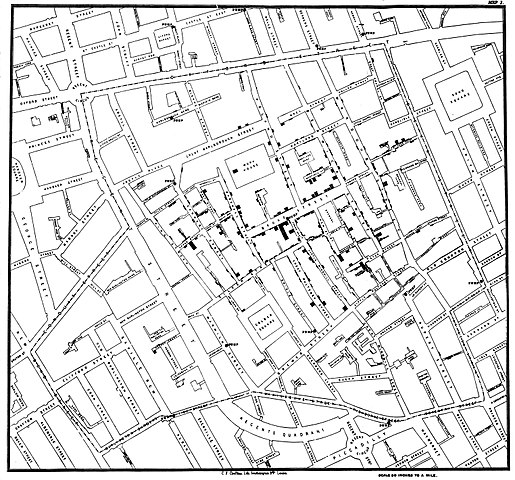
Figure 2. Original map by John Snow showing the clusters of cholera cases in the London epidemic of 1854, drawn and lithographed by Charles Cheffins. Image Public Domain, from Wikipedia

Snow’s work and dataset can be viewed and thanks to Paul Lindman and others, the work can be expanded: for example, define areas around pumps by walking distance (Fig 3). The R package is cholera. Figure 2 shows a plot like Snow’s annotated map.cholera.

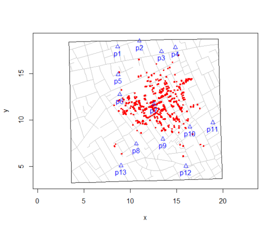
Figure 3. Plot of Snow’s London using R cholera package. Triangles marked with p1-p13 represent public water pumps. Red dots represent cholera cases.

R code to make the plot was

snowMap()

Snow’s ideas about cholera were not accepted in his time and you should recognize that by itself, a cluster map supports both the airborne and waterborne theories. The cholera package contains additional data to help visualize the area, including setting regions by walking distance (Fig 4).

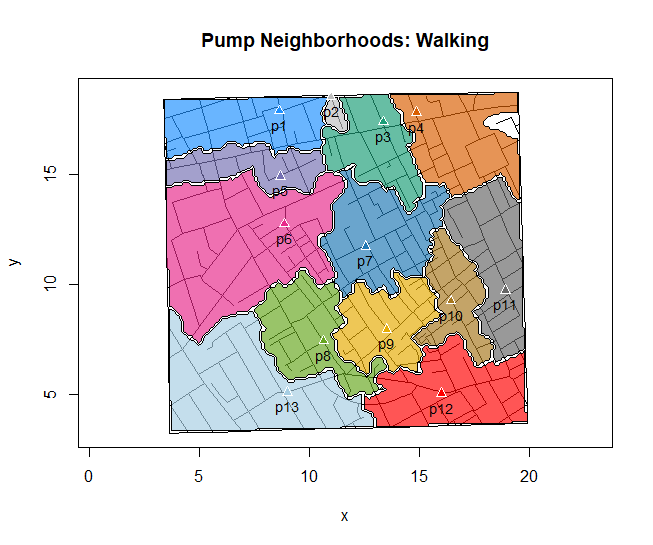
Figure 4. Plot of Snow’s London with walking areas drawn about the 13 water pumps. R cholera package.

R code to make the plot was

plot(neighborhoodWalking(case.set = "expected"), "area.polygons")

Epidemiology of cancer

.

This is an undeveloped section in my book. For now, I’ve listed a number of key landmark studies — a selective and incomplete list — in the history of epidemiology and cancer risk — these would serve well as case studies:

• Tobacco as a carcinogen
  • Doll R, Hill AB. Smoking and carcinoma of the lung; preliminary report. Br Med J 1950; 2: 739–748
  • Fontham ET, Correa P, Wu-Williams A, Reynolds P, Greenberg RS, Buffler PA, Chen VW, Boyd P, Alterman T, Austin DF, Liff J, Greenberg SD. Lung cancer in non-smoking women: a multicenter case-control study. Cancer Epidemiol Biomarkers Prev 1991;1:35-43
• Diet and cancer risk
  • Kolonel LN, Hankin JH, Lee J, Chu SY, Nomura AM, Hinds MW. Nutrient intakes in relation to cancer incidence in Hawaii. Br J Cancer 1981;44:332-339.
• Obesity, exercise, and cancer risk
  • Calle EE, Rodriguez C, Walker-Thurmond K, Thun MJ. Overweight, Obesity, and Mortality from Cancer in a Prospectively Studied Cohort of U.S. Adults. N Engl J Med 2003;348:1625-1638.
• Hormones and cancer risk
  • Marchbanks PA, McDonald JA, Wilson HG, Folger SG, Mandel MG, Daling JR, Bernstein L, Malone KE, Ursin G, Strom BL, Norman SA, Wingo PA, Burkman RT, Berlin JA, Simon MS, Spirtas R, Weiss LK. Oral contraceptives and the risk of breast cancer. New Engl J Med 2002;346(26):2025-2032.
• Cancer risk and occupations
  • absence of cervical cancer but high incidence of breast cancer in nuns (Ramazzini, 1713)
  • cancer of the scrotums among chimney sweeps of London (Pott, 1775)
  • Silverman DT, Hoover RN, Mason TJ, Swanson GM. Motor exhaust-related occupations and bladder cancer. Cancer Res 1986;46:2113-2116.

Please see review by Greenwald and Dunn (2009).

Questions

.

1. Find and copy definitions for “big data” and “data mining” from (a) one peer-reviewed, primary source (e.g., search Google Scholar), (b) one peer-reviewed, secondary source (e.g., search Google Scholar), and (c) Wikipedia. From these three sources, write your own definitions for big data processing and data mining.
2. For each of the statisticians listed identify at least one statistical test attributed to their work. For starters, Francis Galton is known for “regression.” Wikipedia is a pretty good source to start with. 
3. Another open ended assignment: expand my example of landmark studies (also called pivotal or seminal studies) in epidemiology of cancer to a subject of your own interest. For example, vaccination and communicable diseases like polio.

Chapter 2 contents

.

• Introduction
• Why biostatistics?
• Why do we use R Software?
• A brief history of (bio)statistics
• Experimental Design and rise of statistics in medical research
• Scientific method and where statistics fits
• Statistical reasoning
• Chapter 2 – References and suggested reading