14.4 – Randomized block design

Introduction

Randomized Block Designs and Two-Factor ANOVA

In previous lectures, we have introduced you to the standard factorial ANOVA, which may be characterized as being crossed, balanced, and replicated. We expect additional factors (covariates) may contribute to differences among our experimental units, but rather than testing them — which would increase need for additional experimental units because of increased number of groups to test — we randomize our subjects. Randomization is intended to disrupt trends of confounding variables (aka covariates). If the resulting experiment has missing values (see Chapter 5), then we can say that the design is partially replicated; if only one observation is made per group, then the design is not replicated — and perhaps, not very useful!!

A special type of Two-factor ANOVA which includes a “blocking” factor and a treatment factor.

Randomization is one way to control for “uninteresting” confounding factors. Clearly, there will be scenarios in which randomization is impossible. For example, it is impossible to randomly assign subjects to The blocking factor is similar to the 10.3 – Paired t-test. In the paired t-test we had two individuals or groups that we paired (e.g. twins). One specific design is called the Randomized Block Design and we can have more than 2 members in the group. We arrange the experimental units into similar groups, i.e., the blocking factor. Examples of blocking factors may include day (experiments are run over different days), location (experiments may be run at different locations in the laboratory), nucleic acid kits (different vendors), operator (different assistants may work on the experiments), etcetera.

In general we may not be directly interested in the blocking factor. This blocking factor is used to control some factor(s) that we suspect might affect the response variable. Importantly, this has the effect of reducing the sums of squares by an amount equal to the sums of squares for the block. If variability removed by the blocking is significant, Mean Square Error (MSE) will be smaller, meaning that the F for treatment will be bigger — meaning we have a more powerful ANOVA than if we had ignored the blocking.

Statistical Testing in Randomized Block Designs

“Blocks” is a Random Factor because we are “sampling” a few blocks out of a larger possible number of blocks. Treatment is a Fixed Factor, usually.

The statistical model is

The Sources of Variation are simpler than the more typical Two-Factor ANOVA because we do not calculate all the sources of variation –  the interaction is not tested! (Table 1).

Table 1. Sources of variation for a two-way ANOVA, randomized block design

Sources of Variation & Sum of Squares	DF	Mean Squares

Critical Value F_{0.05(2), (a – 1), (Total DF – a – b)}

In the exercise example above: Factor A = exercise or management plan.

Notice that we do not look at the interaction MS or the Blocking Factor (typically).

Learn by doing

Rather than me telling you, try on your own. We’ll begin with a worked example, then proceed to introduce you to three problems. Click here (Ch 14.8)for general discussion of Rcmdr and linear models for models other than the standard 2-way ANOVA (Chapter 14.8).

Worked example

Wheel running by mice is a standard measure of activity behavior. Even wild mice will use wheels (Meijer and Roberts 2014). For example, we conduct a study of family parity to see if offspring from the first, second, or third sets of births from wheel-running behavior in mice (total revs per 24 hr period). Each set of offspring from a female could be treated as a block. Data are for 3 female offspring from each pairing. This type of data set would look like this:

Table 2. Wheel running behavior by three offspring from each of three birth cohorts among four maternal sets (moms).

Thus, there were nine offspring for each female mouse (Dam1 – Dam4), three offspring per each of three litters of pups. The litters are the blocks. We need to get the data stacked to run in R. I’ve provided the dataset for you, scroll to end of this page or click here.

Question 1. Describe the problem and identify the treatment and blocking factors.

Answer. Each female has three litters. We’re primarily interested in genetics (and maternal environment) of wheel running behavior, which is associated with the moms (Treatment factor). The questions is whether there is an effect of birth parity on wheel running behavior. Offspring of a first-time mother may experience different environment than offspring of experienced mother. In this case, parity effects is an interesting question, nevertheless, blocking is the appropriate way to handle this type of problem.

Question 2. What is the statistical model?

Answer. Response variable, Y, is wheel running. Let α the effect of Dam and β the birth cohorts (i.e., the blocking effect).

Question 3. Test the model.

Answer. We fit the main effects, Dam and Block Fig 1.

Rcmdr: Statistics → Fit models → Linear model

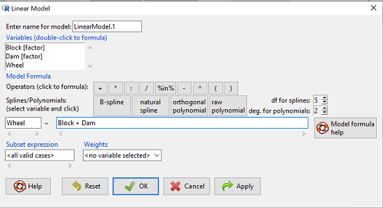
Figure 1. Screenshot Rcmdr Linear Model menu.

then run the ANOVA summary to get the ANOVA table. Rcmdr: Models →  Hypothesis tests → ANOVA table.

Output

Anova Table (Type II tests)

Response: Wheel
           Sum Sq  Df  F value    Pr(>F) 
Dam       1467020   3   4.4732   0.01036 * 
Block     1672166   2   7.6482   0.00207 **
Residuals 3279544  30

Question 4.  Conclusions?

Answer. The null hypotheses are:

Treatment factor: Offspring of the different dams have same wheel running activity of offspring.

Blocking factor: No effect of litter parity on wheel running activity of offspring.

Both the treatment factor (p = 0.01036) and the blocking factor (p = 0.00207) were statistically significant.

Try on your own

Problem 1.

Or we might want to measure the Systolic Blood Pressure of individuals that are on different exercise regimens. However, we are not able to measure all the individuals on the same day at the same time. We suspect that time of day and the day of the year might effect an individuals blood pressure. Given this constraint, the best research design in this circumstance is to measure one individual on each exercise regime at the same time. These different individuals will then be in the same “block” because they share in common the time that their blood pressure was measured. This type of data set would look like this (Table 2):

Table 2. Simulated blood pressure of five subjects on three different exercise regimens.†

Let’s make a line graph to help us visualize trends (Fig 2).

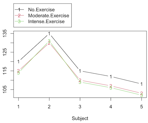
Figure 2. Line graph of data presented in Table 2.

Question 1. Describe the problem and identify the treatment and blocking factors.

Question 2. What is the statistical model?

Question 3. Test the model.

Question 4.  Conclusions?

†You’ll need to arrange the data like the data set for the worked example.

Problem 2.

Another example in conservation biology or agriculture. There may be three different management strategies for promoting the recovery of a plant species. A good research design would be to choose many plots of land (blocks) and perform each treatment (management strategy) on a portion of each plot of land (block). A researcher would start with an equal number of plantings in the plots and see how many grew. The plots of land (blocks) share in common many other aspects of that particular plot of land that may effect the recovery of a species.

Table 3. Growth of plants in 5 different plots subjected to one of three management plans (simulated data set).†

†You’ll need to arrange the data the same arrangement as for the worked example.

These are examples of Two-Factor ANOVA but we are usually only interested in the treatment Factor. We recognize that the blocking factor may contribute to differences among groups and so wish to control for the fact that we carried out the experiments at different times (e.g., seasons) or at different locations (e.g., agriculture plots)

Question 1. Describe the problem and identify the treatment and blocking factors. Make a line graph to help visualize.

Question 2. What is the statistical model?

Question 3. Test the model.

Question 4.  Conclusions?

Repeated-Measures Experimental Design

If multiple measures are taken on the same individual, then we have a repeated-measures experiment. This is a Randomized Block Design. In other words, each animal gets all levels of a treatment (assigned randomly). Thus, samples (individuals) are not independent and the analysis needs to take this into account. Just like for paired-T tests, one can imagine a number of experiments in biomedicine that would conform to this design.

Problem 3.

The data are total blood cholesterol levels for 7 individuals given 3 different drugs (from example given in Zar 1999, Ex 12.5, pp. 257-258).

Table 5. Repeated measures of blood cholesterol levels of seven subjects on three different drug regimens.†

†You’ll need to arrange the data like the data set for the worked example.

Question 1: Is there an interaction term in this design? Make a line graph to help visualize.

Question 2: Are individuals a fixed or a random effect?

Question 2. What is the statistical model?

Question 3. Test the model. Note that we could have done the experiment with 21 randomly selected subjects and a one-factor ANOVA. However, the repeated measures design is best IF there is some association (“correlation”) between the data in each row. The computations are identical to the randomized block analysis.

Question 4.  Conclusions?

Problem 4.

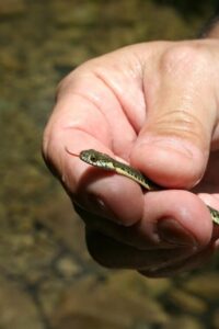
Figure 3. Juvenile garter snake, image from GetArchive, public domain.

Here is a second example of a repeated measures design experiment. Garter snakes (Fig 3) respond to odor cues to find prey. Snakes use their tongues to “taste” the air for chemicals, and flick their tongues rapidly when in contact with suitable prey items, less frequently for items not suitable for prey. In the laboratory, researchers can test how individual snakes respond to different chemical cues by presenting each snake with a swab containing a particular chemical. The researcher then counts how many times the snake flicks its tongue in a certain time period (data presented p. 301, Glover and Mitchell 2016).

Table 6. Tongue flick counts of naïve newborn snakes to extracts†

†You’ll need to arrange the data like the data set for the worked example.

Question 1. Describe the problem and identify the treatment and blocking factors. Make a line graph to help visualize.

Question 2. What is the statistical model?

Question 3. Test the model.

Question 4.  Conclusions?

Additional questions

1. The advantage of a randomized block design over a completely randomized design is that we may compare treatments by using ________________ experimental units.
   A. randomly selected
   B. the same or nearly the same
   C. independent
   D. dependent
   E. All of the above
2. Which of the following is NOT found in an ANOVA table for a randomized block design?
   A. Sum of squares due to interaction
   B. Sum of squares due to factor 1
   C. Sum of squares due to factor 2
   D. None of the above are correct
3. A clinician wishes to compare the effectiveness of three competing brands of blood pressure medication. She takes a random sample of 60 people with high blood pressure and randomly assigns 20 of these 60 people to each of the three brands of blood pressure medication. She then measures the decrease in blood pressure that each person experiences. This is an example of (select all that apply)
   A. a completely randomized experimental design
   B. a randomized block design
   C. a two-factor factorial experiment
   D. a random effects or Type II ANOVA
   E. a mixed model or Type III ANOVA
   F. a fixed effects model or Type I ANOVA
4. A clinician wishes to compare the effectiveness of three competing brands of blood pressure medication. She takes a random sample of 60 people with high blood pressure and randomly assigns 20 of these 60 people to each of the three brands of blood pressure medication. She then measures the blood pressure before treatment and again 6 weeks after treatment for each person. This is an example of (select all that apply)
   A. a completely randomized experimental design
   B. a randomized block design
   C. a two-factor factorial experiment
   D. a random effects or Type II ANOVA
   E. a mixed model or Type III ANOVA
   F. a fixed effects model or Type I ANOVA

Data sets used in this page

Problem 1 data set

Chapter 14 contents

• Introduction
• Crossed, balanced, fully replicated
• Sources of variation
• Fixed effects, Random effects
• Randomized block design
• Nested designs
• Some other ANOVA designs
• Rcmdr Multiway ANOVA
• More on the linear model in Rcmdr
• References and suggested readings