20.3 – Baseline correction

Introduction
Many applications, numerous examples
Statistical considerations
R code
Examples
Questions
References
Chapter 20 contents

draft

Introduction

Signal processing is the analysis and manipulation of signals to extract meaningful information and improve data quality. signal processing is a crucial pre-processing step before analysis, as it involves cleaning and preparing raw data to improve its quality and highlight important features for accurate analysis. Common pre-processing tasks include filtering noise, filling in missing data, and feature extraction, all of which are done before the main analytical steps like feature extraction and classification can be performed.

A baseline refers to an initial measurement before an intervention. A starting point. Provides an objective comparison to judge whether or not an intervention has led to change.

Baseline drift is a gradual, slow shift in the signal’s zero-point over time, while intensity drift is a more general term for a change in a peak’s amplitude, often due to baseline changes. Noise is rapid, random fluctuation that obscures the signal itself. The key differences lie in their speed and effect: drift is a slow, low-frequency, long-term issue that shifts the entire baseline, whereas noise is a fast, high-frequency, short-term issue that adds random variation to the signal

For measures conducted over time, a baseline correction may be applied during initial data processing to correct for signal distortion, background noise, or baseline drift — the gradual change over time in what is expected to be measurement of an unchanging signal.

Note 1: Signal distortion is an unwanted change to the original signal’s waveform, while background noise is an unrelated, external signal that is added to the original signal.

Many applications, numerous examples.

Quantitative PCR, qPCR: baseline correction is the process of identifying and subtracting the background fluorescence noise from the early cycles of a real-time PCR run to accurately measure the signal from specific DNA amplification (see Ruijter et al 2009).

Chromatography: baseline correction is a technique to remove background noise and drift from a chromatogram to make peaks more visible and accurate for analysis (see Niezen et al 2022).

Standard and basal metabolic rate by indirect calorimetry: baseline drift is an error where the instrument’s signal gradually changes over time, independent of the subject’s actual oxygen consumption ( $\dot{V}O_{2}$ ), while baseline correction is a data processing technique used to computationally adjust the recorded data to counteract this drift and improve accuracy (see Hayes et al 1992; Lighton 2017).

Colorimetric spectrometry: baseline drift is an unwanted phenomenon where the signal’s baseline gradually shifts over time or wavelength due to instrumental or environmental factors, while baseline correction is a data processing technique used to computationally remove this drift and other background noise from the measured spectrum.

Statistical considerations

When processing a biological signal such as an electromyogram (EMG), it’s important to remember that even the baseline—the part of the recording where we assume “nothing is happening” — is only an estimate of the true baseline noise level. To account for this, choose two kinds of time windows: a baseline window (before the event of interest) and a signal window (during the activity you want to measure).

Note 1: In signal processing, a window function’s purpose is to isolate a portion of a signal for analysis and reduce spectral leakage by smoothing the signal’s boundaries.

The goal is to compare these windows in a way that fairly adjusts for natural fluctuations in the baseline. One common approach is a regression-weighted correction, which simply means using a statistical line that represents how the baseline trends upward or downward over time, then adjusting the signal based on that line rather than assuming the baseline is perfectly flat. Another approach is to use a spline, which is a smooth, flexible curve that adapts to gradual changes in the baseline. Splines can correct for slow drifts in the recording without over-correcting the actual signal. Together, these methods help ensure that any “activity” you detect is more likely to be real muscle activation and not just shifts in the baseline.

R code

Package(s):

baseline

Signal

Examples

To illustrate, consider a myogram signal trace (EMG) recorded over several minutes. The trace will show fluctuations in electrical activity over time, which reflects muscle rest, contraction, and relaxation. The trace will exhibit a baseline at rest, spikes or bursts of activity during contractions, and varying levels of intensity depending on the muscle’s effort. An increase in the frequency and amplitude of these spikes indicates a stronger, more forceful contraction, while a period of no activity will show as a flat line. In a real-world scenario with an active muscle or a prolonged recording, the trace is typically corrupted by both noise (high-frequency, random variations) and baseline drift (slow, low-frequency shifts from the zero point). Among several statistics, analyst may calculate from the signal (1) the Root Mean Square (RMS) Amplitude, a measure of the signal’s magnitude and represents the overall intensity of muscle activity, (2) Mean Power Frequency (MPF), or the the frequency domain analysis of myogram signals. The MPF is calculated to assess muscle fatigue (fatigue often causes a shift to lower frequencies), and others (eg, Potvin and Bent 1997, Smilios et al 2010). Principle to the analysis, moving average or LOESS approaches may be used to smooth the data, reduce noise, and identify underlying trends or patterns in muscle activity over the multiple-minute duration.

To demonstrate pre-processing steps to correct for baseline drift, we need a data set. Here, we simulate a couple of myogram-like traces.

R code to simulate myogram data with baseline drift and random walk noise. A random walk tends to wander and works well for simulating biological drift.

# Example
# Define simulation parameters
duration_sec <- 5 # Total duration in seconds
sampling_rate_hz <- 1000 # Sampling rate (1000 Hz = 1 ms interval)
peak_center_time <- 2.5 # Time of the muscle contraction peak
amplitude <- 5 # Peak amplitude of the myogram
drift_magnitude <- 0.01 # Factor to control the magnitude of baseline drift
noise_level_sd <- 0.1 # Standard deviation of the white noise

Generate the data

my_data <- simulate_myogram_with_drift(
duration = duration_sec,
hz = sampling_rate_hz,
peak_time = peak_center_time,
peak_amplitude = amplitude,
drift_factor = drift_magnitude,
noise_sd = noise_level_sd
)
head(my_data)

Plot the simulated data

plot(my_dataSignal, type = 'l', col = 'blue',
main = "Simulated Myogram Data with Baseline Drift",
xlab = "Time", ylab = "Signal Value")
lines(my_dataDrift, col = 'red', lty = 2) # Overlay the drift line
legend("topleft", legend = c("Simulated Myogram", "Baseline Drift"),
col = c("blue", "red"), lty = c(1, 2), cex = 0.8)
# ylim = range(myogram_data, baseline_drift)

which gives us graph like Figure 1.

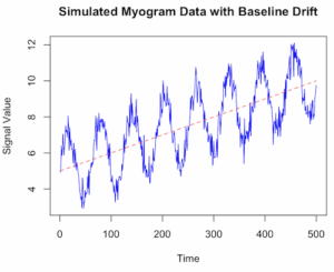
Figure 1. Simulated myogram data with baseline drift.

Alternatively, use ggplot (Fig 2).

library(ggplot2)
ggplot(my_data, aes(x = Time, y = Signal)) +
geom_line(color = “blue”) +
geom_line(aes(y = Drift), color = “red”, linetype = “dashed”, alpha = 0.6) +
geom_line(aes(y = TrueSignal), color = “green”, linetype = “dotted”, alpha = 0.8) +
labs(title = “Simulated Myogram Data with Baseline Drift”,
x = “Time (seconds)”,
y = “Signal Amplitude”) +
theme_minimal() +
scale_color_manual(values = c(“blue”, “red”, “green”),
labels = c(“Total Signal”, “Baseline Drift”, “True Myogram”)) +
theme(legend.position = “bottom”)

# You can access the data for further analysis using the ‘my_data’ data frame
head(my_data)

}

version 2
# R code to simulate myogram data with baseline drift

# 1. Define simulation parameters
set.seed(123) # for reproducibility
n_samples <- 500 # number of data points (time steps)
time <- 1:n_samples
baseline_start <- 5
drift_rate <- 0.01 # slope of the linear drift
signal_amplitude <- 2
noise_sd <- 0.5 # standard deviation of the noise

# 2. Simulate the baseline drift
# A simple linear drift is used here. You could also use a random walk (RW).
baseline_drift <- baseline_start + drift_rate * time

# 3. Simulate the biological signal (myogram activity)
# Using a sinusoidal function as an example of a rhythmic signal
biological_signal <- signal_amplitude * sin(time * 0.1)

# 4. Simulate random noise (white noise)
noise <- rnorm(n_samples, mean = 0, sd = noise_sd)

# 5. Combine all components to get the final simulated myogram data
myogram_data <- baseline_drift + biological_signal + noise

# 6. Create a data frame for plotting and analysis
sim_data <- data.frame(Time = time, Signal = myogram_data)

# 7. Visualize the data using base R graphics or ggplot2
plot(sim_data $Time, sim_data$ Signal, type = ‘l’, col = ‘blue’,
main = “Simulated Myogram Data with Baseline Drift”,
xlab = “Time”, ylab = “Signal Value”, ylim = range(myogram_data, baseline_drift))
lines(sim_data$Time, baseline_drift, col = ‘red’, lty = 2) # Overlay the drift line
legend(“topleft”, legend = c(“Simulated Myogram”, “Baseline Drift”),
col = c(“blue”, “red”), lty = c(1, 2), cex = 0.8)

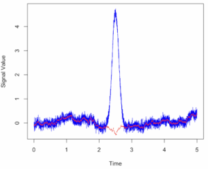
Figure 2. Simulated myogram data with random walk noise and baseline drift.

# You can also use the ggplot2 package for more sophisticated plotting
# install.packages(“ggplot2”)
# library(ggplot2)
# ggplot(sim_data, aes(x = Time, y = Signal)) +
# geom_line(color = “blue”) +
# geom_line(aes(y = baseline_drift), color = “red”, linetype = “dashed”) +
# labs(title = “Simulated Myogram Data with Baseline Drift”,
# y = “Signal Value”) +
# theme_minimal()

Questions

Write up three learning outcomes for this page. Hint: Point your favorite generative AI to this page and ask for help

References

Hayes, J. P., Speakman, J. R., & Racey, P. A. (1992). Sampling bias in respirometry. Physiological Zoology, 65, 604–619.

Lighton, J. R. B. (2017). Limitations and requirements for measuring metabolic rates: A mini review. European Journal of Clinical Nutrition, 71(3), 301–305.

Liland, K. H. (2015). 4S Peak Filling–baseline estimation by iterative mean suppression. MethodsX, 2, 135-140.

Liland, K. H., & Mevik, T. A. B. H. (2011). Optimal baseline correction for multivariate calibration using open-source software. Life Science Instruments, (3), 7.

Niezen, L. E., Schoenmakers, P. J., & Pirok, B. W. J. (2022). Critical comparison of background correction algorithms used in chromatography. Analytica Chimica Acta, 1201, 339605.

Ruijter, J. M., Ramakers, C., Hoogaars, W. M. H., Karlen, Y., Bakker, O., van den Hoff, M. J. B., & Moorman, A. F. M. (2009). Amplification efficiency: Linking baseline and bias in the analysis of quantitative PCR data. Nucleic Acids Research, 37(6), e45.

Potvin, J. R., & Bent, L. R. (1997). A validation of techniques using surface EMG signals from dynamic contractions to quantify muscle fatigue during repetitive tasks. Journal of Electromyography and Kinesiology, 7(2), 131–139.

Smilios, I., Hakkinen, K., & Tokmakidis, S. P. (2010). Power Output and Electromyographic Activity During and After a Moderate Load Muscular Endurance Session. The Journal of Strength and Conditioning Research, 24(8), 2122–2131.

Chapter 20 contents

/MD