20.5 – Time series
Introduction
Time series refers to any measure recorded over time. Stationary time series do not have trends or seasonality, just random (white) noise; differencing, or nonstationary time series do have trends and or seasonality. Stationary time series will not have predictable patterns over the long term, but for us, what this distinction says is that statistics like autocorrelation, the mean and standard deviation remains the same over time. Nonstationary times series can be made stationary by transformation, with taking a differencing approach, subtracting each observation from its preceding one to remove trends and seasonality, one common approach.
All kinds of examples of time series analysis can be made, with stock market price fluctuations (Hamilton 1994) and meteorological forecasting (Mudelsee 2014) as common examples. Time series analysis are also important in clinical situations, for example, analysis of temporal patterns in ECG and blood pressure data, which helps predict risks, monitor patient health, and understand disease trends. In ecology, perhaps the most famous time series data set is the Hudson’s Bay Company fur-trade records, which show a 9- to 11-year predator-prey population cycle between populations of the Canadian lynx (the predator) and the snowshoe hare (the prey) (Krebs et al 1995).
Significant autocorrelation — the correlation between any two observations in a data series separated by a specific time interval or lag — represents the extent to which a time series is correlated with its past values. For example, autocorrelation could measure the association between a person’s heart rate today and its heart rate yesterday, or between its heart rate today and the heart rate from last week. It is not simply the relationship between today’s heart rate and, for instance, today’s environmental temperature. This kind of comparison, between two sets of time series, calls for a cross-correlation or predictive correlation. A cross-correlation measures the correlation between the first series (temperature) and a lagged version of the second series (heart rate some minutes or hours later). Examples of such correlations include our familiar product moment correlation, but generalized across all possible time lags.
Note 1: See RHRV package, the R Heart Rate Variability (HRV) analysis package, for framework to analyze heartbeat, ECG, and other cardiac recordings. See also Chapter 20.3 – Baseline correction for an example of a myogram analysis with baseline drift.
There’s much to the analysis of time series, but one key concept is the moving average. Along with any trend or pattern due to seasonality, time series data are expected to exhibit noise or random variation associated with each point in the series. The moving average is an attempt to smooth out data to reveal underlying trends and are fundamental to seasonal decomposition and forecasting. We calculate a series of averages of different subsets of the data, making it easier to spot long-term patterns by filtering out short-term noise, like fluctuations or outliers.
For example, to calculate the 5-beat moving average of a heartbeat, you would average the last 5 individual heartbeat values. As each new heartbeat is recorded, the oldest one is dropped, and a new average is calculated, creating a smoother trend line that shows a clearer overall picture rather than focusing on individual, potentially spiky, beat-to-beat variations. Rate-responsive or adaptive pacemakers use moving averages to determine the appropriate pacing rate. This helps provide a smoother and more stable heart rate response to the patient’s activity.
Note 2: For some really cool work on adaptive pacemakers, see Kumar et al 2018.
This statistical approach should sound familiar — we introduced without much fanfare use of LOESS (Locally Estimated Scatterplot Smoothing) to smooth data to improve pattern detection in Chapter 4.5 and Chapter 17.4. While a moving average takes average of a fixed number of recent data points, LOESS is a more powerful non-parametric regression technique that fits local polynomial regressions to subsets of the data to create a smooth curve.
In time series analysis, the autocorrelation function (ACF) measures the linear relationship between a time series and a lagged version of itself. It quantifies how correlated a series is with its past values ( ) and
) and  ), where
  is the lag or time interval. An ACF plot, or correlogram, visually displays these correlation coefficients at different lags to help identify patterns, assess randomness, and determine appropriate time series models like ARIMA. ACF is related to moving averages because the ACF plot helps to identify the order of a moving average model, which depends on the ACF’s behavior at different lags.
Note 3: A time-series plot shows how a single variable changes over time, while an ACF (Autocorrelation Function) plot visualizes the correlation between a time series and a lagged version of itself.
Like many pages in Mike’s Biostatistics Book, this page only begins to introduce the subject. For a more thorough introduction, see Introduction to Time Series Analysis, NIST. See also the text by Shumway and Stoffer (2025).
ARIMA and ARMA models
ARIMA and ARMA models are fundamental tools for analyzing time series data in biostatistics, especially when the goal is to understand temporal patterns or forecast future values. An ARMA model combines two ideas: autoregression (AR), where the current value depends on previous values, and moving average (MA), where the current value depends on previous error terms. An ARIMA model extends this by adding differencing—the “I” for Integrated—which helps remove trends and make the series stationary. These models are widely used in public health, epidemiology, and biological monitoring because many variables (e.g., infection rates, physiological signals) show correlation over time.
Note 4: We introduced ARMA models in our Generalized Linear models introduction, Chapter 18.4.
Both ARMA and ARIMA models rely on the concepts of lagged dependence and error smoothing, but ARIMA is more flexible because it explicitly accommodates nonstationary data. An ARMA(p, q) model is appropriate when the time series is already stationary or has been preprocessed to remove trend and seasonality.  is the autoregressive order, the number of lagged observations used to forecast the current value, and
  is the moving average order, the number of lagged forecast errors included in the model.
In contrast, ARIMA(p, d, q) includes a differencing parameter  that automatically transforms the series to stationarity before fitting the ARMA structure. Thus, ARIMA models are typically used for data with a clear trend or evolving mean, while ARMA models are a subset applied to stable series without differencing. In practice, ARIMA is more commonly applied because real-world biological and clinical time series often exhibit trends.
R code
In R, ARMA and ARIMA models can be fit using the forecast or stats packages. The code below shows simple examples of each using a generic time series object  . An ARMA(2,1) model can be fit with:
arma_model <- arima(y, order = c(2, 0, 1))
summary(arma_model)
where the middle “0” indicates no differencing. For an ARIMA(1,1,1) model, which includes first differencing to remove trend, the code is:
arima_model <- arima(y, order = c(1, 1, 1))
summary(arima_model)
ccc
R packages
To conduct time series analysis we can use built in functions like ts() and decompose(). HoltWinters() also useful, now part of stats. Lots of specialized time series packages with advanced features, including forecast, timeSeries (Financial time series), season (Seasonal analysis of health data), and many others. For a more extensive package, see asta, which was designed to accompany the excellent book, now in its 5th edition, Time Series Analysis and its Applications: With R Examples, by Shumway and Stoffer (2025).
Note 4: Caution — newer versions of R have HoltWinters() and related functions included with base package stats.
Rcmdr package for time series was RcmdrPlugin.epack , removed from CRAN as of 2018.
For up-to-date listing of time series packages, see https://cran.r-project.org/web/views/TimeSeries.html
Time series data sets included in R and Rcmdr
R Code
data(co2, package="datasets")
co2 <- as.data.frame(co2)
#convert to time series data type with ts()
tCO2 <- ts(co2,frequency=12,start=c(1959),end=c(1997))
plot.ts(tCO2)
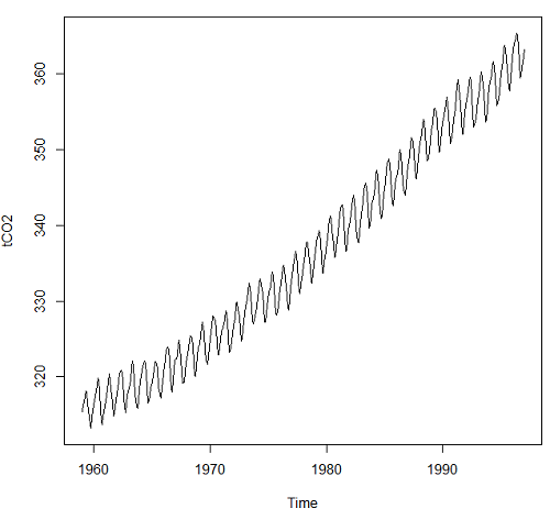
Figure 1. Time series plot of CO2 data set, the Keeling curve, from package datasets, comes with Rcmdr installation.
Other datasets included with R
carData::Arrests
carData::Bfox
carData::CanPop
Example
Get up-to-date CO2 data from NOAA as text file. Download to your computer, load and clean in your favorite spreadsheet app. Months came as numbers 1,2,3, etc., I changed to text, Jan, Feb, Mar, etc. I grabbed three columns: year, month, ppm for import to R.
head(maunaLoa)
R output
> head(maunaLoa)
  year month  ppm
1 1958 Mar 315.70
2 1958 Apr 317.45
3 1958 May 317.51
4 1958 Jun 317.24
5 1958 Jul 315.86
6 1958 Aug 314.93
However, it turns out the time series functions are easiest to work if only the ppm data are included.
tCO2 <- ts(maunaLoa[,"ppm"],frequency=12,start=c(1958,3),end=c(2020,10))
head(tCO2)
R output
> head(tCO2)
        Mar    Apr    May    Jun    Jul    Aug
1958 315.70 317.45 317.51 317.24 315.86 314.93
Get our plot (Figure 2).
plot(tCO2)
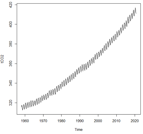
Figure 2. CO2 ppm monthly average data from NOAA, last data October 2020.
Seasonal time series comes with a trend component, a seasonal component, and a random component.
R code
dectCO2 <- decompose(tCO2)
head(dectCO2)
plot(dectCO2)
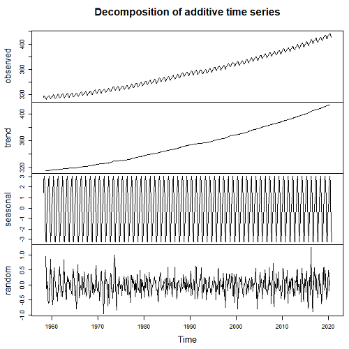
Figure 3. Observed (panel, top), trends over time (panel, second from top), seasonal changes (panel, second from bottom), and random error (panel, bottom).
Forecasting
Excellent resource at https://otexts.com/fpp2/
Exponential smoothing, weighted averages of past observations, weighted so that more recent observations are more influential.
Holt-Winters method extracts seasonal component (additive or multiplicative).
#set start value to value of first observation
tCO2cast <- HoltWinters(tCO2, l.start=315.42)
#Predict for next ten years. Because frequency in ts() was monthly, ten years is h=120
forecastCO2 <- forecast(tCO2cast, h=120)
plot(forecastCO2, fcol="red")
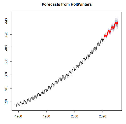
Figure 4. Data in black, predicted values in red (additive) shaded by confidence interval.
Questions
- Write up three learning outcomes for this page. Hint: Point your favorite generative AI to this page and ask for help.
- For the co2 dataset included in Rcmdr (co2, datasets), obtain forecast for year 2020 and compare against actual 2020 data (see Figure 2).
- Positive clinical samples between September 2015 and November 2020 for flu virus in the USA are provided in the data set below (scroll or click here). The frequency of observations was weekly. Apply
decompose()and obtain the seasonal and trend components of the data set. Which month does the peak positive sample occur? - Total pounds of fish (variable = Pounds) and pounds of Akule and Opelu (variable = Akule.Opelu) caught by commercial industry in Hawaiʻi, from 2000 to 2018 are provided in the data set below (scroll or click here). Apply
decompose()and obtain the seasonal and trend components of the data set for Total pounds and again for Akule (Selar crumenophthalmus) and Opelu (Decapterus macarellus). Is there evidence for trends, and if so, describe the trend. Is there evidence of seasonality? If so, which month did peak fishing occur?
Quiz Chapter 20.5
Time series
References and suggested reading
Hamilton, J. D. (1994). Time Series Analysis. Princeton University Press.
Krebs, C. J., Boutin, S., Boonstra, R., Sinclair, A. R. E., Smith, J. N. M., Dale, M. R. T., Martin, K., & Turkington, R. (1995). Impact of food and predation on the snowshoe hare cycle. Science, 269(25 August), 1112–1115.
Kumar, A., Komaragiri, R., & Kumar, M. (2018). From Pacemaker to Wearable: Techniques for ECG Detection Systems. Journal of Medical Systems, 42(2), 34.
Chapter 6.4. Introduction to Time Series Analysis, in NIST/SEMATECH e-Handbook of Statistical Methods, https://www.itl.nist.gov/div898/handbook/index.htm, (first reviewed by Mike in 2019).
Mudelsee, M. (2016). Climate time series Classical statistics and bootstrap methods (2nd ed., Vol. 51). Springer.
Shumway, R. H., & Stoffer, D. S. (2025). Time Series Analysis and Its Applications: With R Examples (5th ed.). Springer.
Data set this page
Flu, extracted 28 Nov 2020 from https://gis.cdc.gov/grasp/fluview/fluportaldashboard.html
| Year | Date | Week | Positive |
|---|---|---|---|
| 2015 | 09/28/15 | 40 | 1.056 |
| 2015 | 10/05/15 | 41 | 1.297 |
| 2015 | 10/12/15 | 42 | 1.109 |
| 2015 | 10/19/15 | 43 | 1.108 |
| 2015 | 10/26/15 | 44 | 1.123 |
| 2015 | 11/02/15 | 45 | 1.382 |
| 2015 | 11/09/15 | 46 | 1.193 |
| 2015 | 11/16/15 | 47 | 1.385 |
| 2015 | 11/23/15 | 48 | 1.395 |
| 2015 | 11/30/15 | 49 | 1.475 |
| 2015 | 12/07/15 | 50 | 2.512 |
| 2015 | 12/14/15 | 51 | 2.287 |
| 2015 | 12/21/15 | 52 | 2.46 |
| 2016 | 01/04/16 | 1 | 2.931 |
| 2016 | 01/11/16 | 2 | 4.254 |
| 2016 | 01/18/16 | 3 | 5.485 |
| 2016 | 01/25/16 | 4 | 6.96 |
| 2016 | 02/01/16 | 5 | 9.699 |
| 2016 | 02/08/16 | 6 | 12.549 |
| 2016 | 02/15/16 | 7 | 15.536 |
| 2016 | 02/22/16 | 8 | 18.362 |
| 2016 | 02/29/16 | 9 | 21.11 |
| 2016 | 03/07/16 | 10 | 23.645 |
| 2016 | 03/14/16 | 11 | 19.972 |
| 2016 | 03/21/16 | 12 | 18.471 |
| 2016 | 03/28/16 | 13 | 16.227 |
| 2016 | 04/04/16 | 14 | 14.016 |
| 2016 | 04/11/16 | 15 | 13.236 |
| 2016 | 04/18/16 | 16 | 12.346 |
| 2016 | 04/25/16 | 17 | 10.262 |
| 2016 | 05/02/16 | 18 | 8.121 |
| 2016 | 05/09/16 | 19 | 6.686 |
| 2016 | 05/16/16 | 20 | 5.811 |
| 2016 | 05/23/16 | 21 | 4.719 |
| 2016 | 05/30/16 | 22 | 3.06 |
| 2016 | 06/06/16 | 23 | 3.02 |
| 2016 | 06/13/16 | 24 | 1.829 |
| 2016 | 06/20/16 | 25 | 1.712 |
| 2016 | 06/27/16 | 26 | 1.223 |
| 2016 | 07/04/16 | 27 | 0.903 |
| 2016 | 07/11/16 | 28 | 0.869 |
| 2016 | 07/18/16 | 29 | 0.849 |
| 2016 | 07/25/16 | 30 | 0.782 |
| 2016 | 08/01/16 | 31 | 0.934 |
| 2016 | 08/08/16 | 32 | 0.901 |
| 2016 | 08/15/16 | 33 | 0.803 |
| 2016 | 08/22/16 | 34 | 1.405 |
| 2016 | 08/29/16 | 35 | 1.678 |
| 2016 | 09/05/16 | 36 | 1.461 |
| 2016 | 09/12/16 | 37 | 1.513 |
| 2016 | 09/19/16 | 38 | 1.741 |
| 2016 | 09/26/16 | 39 | 1.784 |
| 2016 | 10/03/16 | 40 | 1.57 |
| 2016 | 10/10/16 | 41 | 1.359 |
| 2016 | 10/17/16 | 42 | 1.403 |
| 2016 | 10/24/16 | 43 | 1.509 |
| 2016 | 10/31/16 | 44 | 1.916 |
| 2016 | 11/07/16 | 45 | 2.201 |
| 2016 | 11/14/16 | 46 | 2.576 |
| 2016 | 11/21/16 | 47 | 3.348 |
| 2016 | 11/28/16 | 48 | 3.319 |
| 2016 | 12/05/16 | 49 | 4.26 |
| 2016 | 12/12/16 | 50 | 6.683 |
| 2016 | 12/19/16 | 51 | 10.782 |
| 2016 | 12/26/16 | 52 | 13.999 |
| 2017 | 01/02/17 | 1 | 13.344 |
| 2017 | 01/09/17 | 2 | 15.373 |
| 2017 | 01/16/17 | 3 | 18.287 |
| 2017 | 01/23/17 | 4 | 18.53 |
| 2017 | 01/30/17 | 5 | 21.422 |
| 2017 | 02/06/17 | 6 | 24.153 |
| 2017 | 02/13/17 | 7 | 24.512 |
| 2017 | 02/20/17 | 8 | 24.725 |
| 2017 | 02/27/17 | 9 | 19.772 |
| 2017 | 03/06/17 | 10 | 19.271 |
| 2017 | 03/13/17 | 11 | 19.034 |
| 2017 | 03/20/17 | 12 | 19.711 |
| 2017 | 03/27/17 | 13 | 18.482 |
| 2017 | 04/03/17 | 14 | 15.425 |
| 2017 | 04/10/17 | 15 | 12.74 |
| 2017 | 04/17/17 | 16 | 9.696 |
| 2017 | 04/24/17 | 17 | 6.768 |
| 2017 | 05/01/17 | 18 | 5.918 |
| 2017 | 05/08/17 | 19 | 5.333 |
| 2017 | 05/15/17 | 20 | 4.863 |
| 2017 | 05/22/17 | 21 | 4.352 |
| 2017 | 05/29/17 | 22 | 4.165 |
| 2017 | 06/05/17 | 23 | 3.386 |
| 2017 | 06/12/17 | 24 | 3.062 |
| 2017 | 06/19/17 | 25 | 2.649 |
| 2017 | 06/26/17 | 26 | 2.534 |
| 2017 | 07/03/17 | 27 | 2.178 |
| 2017 | 07/10/17 | 28 | 2.164 |
| 2017 | 07/17/17 | 29 | 1.839 |
| 2017 | 07/24/17 | 30 | 1.806 |
| 2017 | 07/31/17 | 31 | 1.948 |
| 2017 | 08/07/17 | 32 | 1.9 |
| 2017 | 08/14/17 | 33 | 1.343 |
| 2017 | 08/21/17 | 34 | 1.434 |
| 2017 | 08/28/17 | 35 | 1.935 |
| 2017 | 09/04/17 | 36 | 1.888 |
| 2017 | 09/11/17 | 37 | 1.896 |
| 2017 | 09/18/17 | 38 | 1.669 |
| 2017 | 09/25/17 | 39 | 1.703 |
| 2017 | 10/02/17 | 40 | 2.202 |
| 2017 | 10/09/17 | 41 | 2.09 |
| 2017 | 10/16/17 | 42 | 2.176 |
| 2017 | 10/23/17 | 43 | 2.583 |
| 2017 | 10/30/17 | 44 | 3.607 |
| 2017 | 11/06/17 | 45 | 4.245 |
| 2017 | 11/13/17 | 46 | 5.3 |
| 2017 | 11/20/17 | 47 | 7.088 |
| 2017 | 11/27/17 | 48 | 7.305 |
| 2017 | 12/04/17 | 49 | 10.745 |
| 2017 | 12/11/17 | 50 | 15.355 |
| 2017 | 12/18/17 | 51 | 22.777 |
| 2017 | 12/25/17 | 52 | 25.386 |
| 2018 | 01/01/18 | 1 | 25.365 |
| 2018 | 01/08/18 | 2 | 26.942 |
| 2018 | 01/15/18 | 3 | 27.034 |
| 2018 | 01/22/18 | 4 | 27.37 |
| 2018 | 01/29/18 | 5 | 27.064 |
| 2018 | 02/05/18 | 6 | 26.998 |
| 2018 | 02/12/18 | 7 | 26.117 |
| 2018 | 02/19/18 | 8 | 22.616 |
| 2018 | 02/26/18 | 9 | 18.487 |
| 2018 | 03/05/18 | 10 | 15.694 |
| 2018 | 03/12/18 | 11 | 15.581 |
| 2018 | 03/19/18 | 12 | 15.328 |
| 2018 | 03/26/18 | 13 | 15.114 |
| 2018 | 04/02/18 | 14 | 12.689 |
| 2018 | 04/09/18 | 15 | 11.249 |
| 2018 | 04/16/18 | 16 | 9.398 |
| 2018 | 04/23/18 | 17 | 7.999 |
| 2018 | 04/30/18 | 18 | 6.259 |
| 2018 | 05/07/18 | 19 | 4.393 |
| 2018 | 05/14/18 | 20 | 3.166 |
| 2018 | 05/21/18 | 21 | 2.39 |
| 2018 | 05/28/18 | 22 | 1.529 |
| 2018 | 06/04/18 | 23 | 1.577 |
| 2018 | 06/11/18 | 24 | 1.299 |
| 2018 | 06/18/18 | 25 | 1.023 |
| 2018 | 06/25/18 | 26 | 1.114 |
| 2018 | 07/02/18 | 27 | 1.003 |
| 2018 | 07/09/18 | 28 | 0.916 |
| 2018 | 07/16/18 | 29 | 1.053 |
| 2018 | 07/23/18 | 30 | 0.995 |
| 2018 | 07/30/18 | 31 | 0.954 |
| 2018 | 08/06/18 | 32 | 0.957 |
| 2018 | 08/13/18 | 33 | 0.764 |
| 2018 | 08/20/18 | 34 | 1.336 |
| 2018 | 08/27/18 | 35 | 1.504 |
| 2018 | 09/03/18 | 36 | 1.747 |
| 2018 | 09/10/18 | 37 | 1.687 |
| 2018 | 09/17/18 | 38 | 1.699 |
| 2018 | 09/24/18 | 39 | 1.497 |
| 2018 | 10/01/18 | 40 | 1.749 |
| 2018 | 10/08/18 | 41 | 1.697 |
| 2018 | 10/15/18 | 42 | 1.993 |
| 2018 | 10/22/18 | 43 | 2.055 |
| 2018 | 10/29/18 | 44 | 2.174 |
| 2018 | 11/05/18 | 45 | 2.733 |
| 2018 | 11/12/18 | 46 | 3.157 |
| 2018 | 11/19/18 | 47 | 3.928 |
| 2018 | 11/26/18 | 48 | 3.915 |
| 2018 | 12/03/18 | 49 | 6.232 |
| 2018 | 12/10/18 | 50 | 10.364 |
| 2018 | 12/17/18 | 51 | 14.265 |
| 2018 | 12/24/18 | 52 | 16.352 |
| 2019 | 12/31/18 | 1 | 12.139 |
| 2019 | 01/07/19 | 2 | 12.722 |
| 2019 | 01/14/19 | 3 | 16.317 |
| 2019 | 01/21/19 | 4 | 19.392 |
| 2019 | 01/28/19 | 5 | 22.549 |
| 2019 | 02/04/19 | 6 | 25.134 |
| 2019 | 02/11/19 | 7 | 26.026 |
| 2019 | 02/18/19 | 8 | 26.241 |
| 2019 | 02/25/19 | 9 | 26.074 |
| 2019 | 03/04/19 | 10 | 25.607 |
| 2019 | 03/11/19 | 11 | 26.132 |
| 2019 | 03/18/19 | 12 | 22.481 |
| 2019 | 03/25/19 | 13 | 19.304 |
| 2019 | 04/01/19 | 14 | 14.942 |
| 2019 | 04/08/19 | 15 | 11.909 |
| 2019 | 04/15/19 | 16 | 8.611 |
| 2019 | 04/22/19 | 17 | 5.844 |
| 2019 | 04/29/19 | 18 | 4.82 |
| 2019 | 05/06/19 | 19 | 3.84 |
| 2019 | 05/13/19 | 20 | 3.542 |
| 2019 | 05/20/19 | 21 | 3.42 |
| 2019 | 05/27/19 | 22 | 3.083 |
| 2019 | 06/03/19 | 23 | 2.79 |
| 2019 | 06/10/19 | 24 | 2.316 |
| 2019 | 06/17/19 | 25 | 1.902 |
| 2019 | 06/24/19 | 26 | 2.081 |
| 2019 | 07/01/19 | 27 | 2.429 |
| 2019 | 07/08/19 | 28 | 2.017 |
| 2019 | 07/15/19 | 29 | 2.218 |
| 2019 | 07/22/19 | 30 | 2.377 |
| 2019 | 07/29/19 | 31 | 2.398 |
| 2019 | 08/05/19 | 32 | 2.054 |
| 2019 | 08/12/19 | 33 | 2.082 |
| 2019 | 08/19/19 | 34 | 2.362 |
| 2019 | 08/26/19 | 35 | 3.455 |
| 2019 | 09/02/19 | 36 | 3.097 |
| 2019 | 09/09/19 | 37 | 2.484 |
| 2019 | 09/16/19 | 38 | 2.757 |
| 2019 | 09/23/19 | 39 | 2.744 |
| 2019 | 09/30/19 | 40 | 1.31 |
| 2019 | 10/07/19 | 41 | 1.479 |
| 2019 | 10/14/19 | 42 | 1.552 |
| 2019 | 10/21/19 | 43 | 2.253 |
| 2019 | 10/28/19 | 44 | 3.057 |
| 2019 | 11/04/19 | 45 | 5.163 |
| 2019 | 11/11/19 | 46 | 6.756 |
| 2019 | 11/18/19 | 47 | 9.546 |
| 2019 | 11/25/19 | 48 | 10.939 |
| 2019 | 12/02/19 | 49 | 11.655 |
| 2019 | 12/09/19 | 50 | 16.154 |
| 2019 | 12/16/19 | 51 | 22.533 |
| 2019 | 12/23/19 | 52 | 26.934 |
| 2020 | 12/30/19 | 1 | 23.488 |
| 2020 | 01/06/20 | 2 | 23.119 |
| 2020 | 01/13/20 | 3 | 26.083 |
| 2020 | 01/20/20 | 4 | 28.281 |
| 2020 | 01/27/20 | 5 | 30.147 |
| 2020 | 02/03/20 | 6 | 30.26 |
| 2020 | 02/10/20 | 7 | 29.675 |
| 2020 | 02/17/20 | 8 | 28.322 |
| 2020 | 02/24/20 | 9 | 25.752 |
| 2020 | 03/02/20 | 10 | 22.491 |
| 2020 | 03/09/20 | 11 | 15.813 |
| 2020 | 03/16/20 | 12 | 7.502 |
| 2020 | 03/23/20 | 13 | 2.322 |
| 2020 | 03/30/20 | 14 | 1.031 |
| 2020 | 04/06/20 | 15 | 0.618 |
| 2020 | 04/13/20 | 16 | 0.623 |
| 2020 | 04/20/20 | 17 | 0.218 |
| 2020 | 04/27/20 | 18 | 0.263 |
| 2020 | 05/04/20 | 19 | 0.326 |
| 2020 | 05/11/20 | 20 | 0.306 |
| 2020 | 05/18/20 | 21 | 0.213 |
| 2020 | 05/25/20 | 22 | 0.165 |
| 2020 | 06/01/20 | 23 | 0.34 |
| 2020 | 06/08/20 | 24 | 0.28 |
| 2020 | 06/15/20 | 25 | 0.381 |
| 2020 | 06/22/20 | 26 | 0.282 |
| 2020 | 06/29/20 | 27 | 0.21 |
| 2020 | 07/06/20 | 28 | 0.176 |
| 2020 | 07/13/20 | 29 | 0.376 |
| 2020 | 07/20/20 | 30 | 0.15 |
| 2020 | 07/27/20 | 31 | 0.133 |
| 2020 | 08/03/20 | 32 | 0.176 |
| 2020 | 08/10/20 | 33 | 0.132 |
| 2020 | 08/17/20 | 34 | 0.227 |
| 2020 | 08/24/20 | 35 | 0.315 |
| 2020 | 08/31/20 | 36 | 0.202 |
| 2020 | 09/07/20 | 37 | 0.186 |
| 2020 | 09/14/20 | 38 | 0.4 |
| 2020 | 09/21/20 | 39 | 0.225 |
| 2020 | 09/28/20 | 40 | 0.33 |
| 2020 | 10/05/20 | 41 | 0.401 |
| 2020 | 10/12/20 | 42 | 0.35 |
| 2020 | 10/19/20 | 43 | 0.251 |
| 2020 | 10/26/20 | 44 | 0.201 |
| 2020 | 11/02/20 | 45 | 0.177 |
| 2020 | 11/09/20 | 46 | 0.222 |
Data set in this page
Fish, Hawaiʻi state DLNR, Pounds refers to total catch, Akule.Opelu refers to pounds for the two kinds of fish.
| Year | Month | Pounds | Akule.Opelu |
|---|---|---|---|
| 1999 | Jan | 2064023 | 85331 |
| 1999 | Feb | 2286785 | 89537 |
| 1999 | Mar | 2083789 | 112897 |
| 1999 | Apr | 2446840 | 136301 |
| 1999 | May | 2300842 | 103692 |
| 1999 | Jun | 2340116 | 134432 |
| 1999 | Jul | 2646429 | 138814 |
| 1999 | Aug | 2254408 | 96569 |
| 1999 | Sep | 1926381 | 56598 |
| 1999 | Oct | 2233789 | 76834 |
| 1999 | Nov | 1730672 | 134706 |
| 1999 | Dec | 1762375 | 92255 |
| 2000 | Jan | 1501164 | 147104 |
| 2000 | Feb | 1993373 | 104165 |
| 2000 | Mar | 2220831 | 132028 |
| 2000 | Apr | 2398180 | 119224 |
| 2000 | May | 2557229 | 121268 |
| 2000 | Jun | 2510298 | 145200 |
| 2000 | Jul | 2270954 | 93883 |
| 2000 | Aug | 1912654 | 69107 |
| 2000 | Sep | 1365264 | 65007 |
| 2000 | Oct | 1615117 | 51208 |
| 2000 | Nov | 1388453 | 117493 |
| 2000 | Dec | 1802926 | 121486 |
| 2001 | Jan | 1481810 | 170702 |
| 2001 | Feb | 1496356 | 44575 |
| 2001 | Mar | 1579528 | 101764 |
| 2001 | Apr | 1184591 | 89388 |
| 2001 | May | 2091424 | 124193 |
| 2001 | Jun | 1966886 | 61122 |
| 2001 | Jul | 2113931 | 73266 |
| 2001 | Aug | 1926661 | 29386 |
| 2001 | Sep | 1353429 | 30268 |
| 2001 | Oct | 1338289 | 29577 |
| 2001 | Nov | 1747198 | 80350 |
| 2001 | Dec | 1458336 | 22817 |
| 2002 | Jan | 1517609 | 107406 |
| 2002 | Feb | 1729084 | 31030 |
| 2002 | Mar | 1747985 | 67691 |
| 2002 | Apr | 2109451 | 101043 |
| 2002 | May | 2069921 | 57251 |
| 2002 | Jun | 1640151 | 100501 |
| 2002 | Jul | 1979382 | 87584 |
| 2002 | Aug | 1831678 | 65566 |
| 2002 | Sep | 1734201 | 53162 |
| 2002 | Oct | 1779207 | 93867 |
| 2002 | Nov | 2191825 | 106167 |
| 2002 | Dec | 2576191 | 67881 |
| 2003 | Jan | 1910500 | 49420 |
| 2003 | Feb | 2075168 | 55006 |
| 2003 | Mar | 2245753 | 71616 |
| 2003 | Apr | 1562751 | 102993 |
| 2003 | May | 2440228 | 106600 |
| 2003 | Jun | 1842907 | 101715 |
| 2003 | Jul | 1957279 | 48453 |
| 2003 | Aug | 2143823 | 69130 |
| 2003 | Sep | 1503212 | 74525 |
| 2003 | Oct | 1611779 | 70949 |
| 2003 | Nov | 1668167 | 54004 |
| 2003 | Dec | 2312537 | 43054 |
| 2004 | Jan | 1605595 | 75751 |
| 2004 | Feb | 1705533 | 94864 |
| 2004 | Mar | 2079402 | 120305 |
| 2004 | Apr | 1883704 | 90950 |
| 2004 | May | 1830168 | 111599 |
| 2004 | Jun | 1918622 | 76392 |
| 2004 | Jul | 2029787 | 98937 |
| 2004 | Aug | 1928009 | 72577 |
| 2004 | Sep | 1620224 | 82650 |
| 2004 | Oct | 1854643 | 74587 |
| 2004 | Nov | 1981567 | 59753 |
| 2004 | Dec | 2022272 | 44353 |
| 2005 | Jan | 2088821 | 60972 |
| 2005 | Feb | 2106948 | 59469 |
| 2005 | Mar | 2386327 | 84551 |
| 2005 | Apr | 2122171 | 101099 |
| 2005 | May | 2369953 | 79042 |
| 2005 | Jun | 2342117 | 104814 |
| 2005 | Jul | 2281871 | 71065 |
| 2005 | Aug | 2124303 | 53383 |
| 2005 | Sep | 1734986 | 37195 |
| 2005 | Oct | 1920131 | 48632 |
| 2005 | Nov | 1969506 | 88235 |
| 2005 | Dec | 2323933 | 98768 |
| 2006 | Jan | 1702766 | 50553 |
| 2006 | Feb | 2060204 | 89037 |
| 2006 | Mar | 2244570 | 33916 |
| 2006 | Apr | 2068922 | 74430 |
| 2006 | May | 2164076 | 108689 |
| 2006 | Jun | 1935951 | 89503 |
| 2006 | Jul | 1968513 | 93758 |
| 2006 | Aug | 1741802 | 111080 |
| 2006 | Sep | 1508897 | 44537 |
| 2006 | Oct | 1892535 | 46747 |
| 2006 | Nov | 2208173 | 82938 |
| 2006 | Dec | 1381412 | 42260 |
| 2007 | Jan | 2211384 | 114496 |
| 2007 | Feb | 2391437 | 60618 |
| 2007 | Mar | 2724021 | 94251 |
| 2007 | Apr | 2639245 | 90078 |
| 2007 | May | 3168913 | 129258 |
| 2007 | Jun | 2706972 | 116628 |
| 2007 | Jul | 2523392 | 129345 |
| 2007 | Aug | 2272502 | 88997 |
| 2007 | Sep | 2121837 | 71560 |
| 2007 | Oct | 2472996 | 52915 |
| 2007 | Nov | 3040118 | 107555 |
| 2007 | Dec | 2934174 | 39239 |
| 2008 | Jan | 2656539 | 44672 |
| 2008 | Feb | 3101819 | 35213 |
| 2008 | Mar | 2816846 | 74421 |
| 2008 | Apr | 3064837 | 63355 |
| 2008 | May | 3560993 | 52287 |
| 2008 | Jun | 2920219 | 33685 |
| 2008 | Jul | 2516561 | 31288 |
| 2008 | Aug | 2338205 | 62171 |
| 2008 | Sep | 2314458 | 31311 |
| 2008 | Oct | 2407240 | 42766 |
| 2008 | Nov | 2060666 | 75102 |
| 2008 | Dec | 2329268 | 74508 |
| 2009 | Jan | 2198569 | 44459 |
| 2009 | Feb | 2314764 | 33206 |
| 2009 | Mar | 1846459 | 64879 |
| 2009 | Apr | 2659230 | 36638 |
| 2009 | May | 2692440 | 77011 |
| 2009 | Jun | 2387175 | 49217 |
| 2009 | Jul | 2672895 | 55033 |
| 2009 | Aug | 2174027 | 40398 |
| 2009 | Sep | 2259153 | 51386 |
| 2009 | Oct | 2386749 | 58095 |
| 2009 | Nov | 2081706 | 51798 |
| 2009 | Dec | 2702871 | 55148 |
| 2010 | Jan | 2059964 | 40855 |
| 2010 | Feb | 2632985 | 100598 |
| 2010 | Mar | 2430562 | 39887 |
| 2010 | Apr | 2652013 | 40528 |
| 2010 | May | 2460228 | 71483 |
| 2010 | Jun | 2743053 | 120553 |
| 2010 | Jul | 2278847 | 96315 |
| 2010 | Aug | 2618427 | 62854 |
| 2010 | Sep | 2483861 | 66613 |
| 2010 | Oct | 2503321 | 53353 |
| 2010 | Nov | 2370032 | 104360 |
| 2010 | Dec | 2431047 | 57919 |
| 2011 | Jan | 2527241 | 37755 |
| 2011 | Feb | 2786453 | 51863 |
| 2011 | Mar | 3789076 | 40188 |
| 2011 | Apr | 3148826 | 60494 |
| 2011 | May | 3015187 | 49037 |
| 2011 | Jun | 2718583 | 58380 |
| 2011 | Jul | 2284521 | 43096 |
| 2011 | Aug | 2475519 | 33612 |
| 2011 | Sep | 2461640 | 48697 |
| 2011 | Oct | 2420554 | 49929 |
| 2011 | Nov | 2059769 | 63045 |
| 2011 | Dec | 2882776 | 64430 |
| 2012 | Jan | 2825116 | 42894 |
| 2012 | Feb | 2653892 | 23528 |
| 2012 | Mar | 2544758 | 39839 |
| 2012 | Apr | 3050109 | 47250 |
| 2012 | May | 3264666 | 41357 |
| 2012 | Jun | 2798204 | 56808 |
| 2012 | Jul | 3331174 | 46853 |
| 2012 | Aug | 2864088 | 62682 |
| 2012 | Sep | 2219536 | 33641 |
| 2012 | Oct | 2482162 | 47478 |
| 2012 | Nov | 2545142 | 49232 |
| 2012 | Dec | 3129507 | 35924 |
| 2013 | Jan | 2902748 | 32373 |
| 2013 | Feb | 2388197 | 21922 |
| 2013 | Mar | 2831279 | 41718 |
| 2013 | Apr | 2467444 | 54619 |
| 2013 | May | 3131153 | 57183 |
| 2013 | Jun | 2819983 | 33484 |
| 2013 | Jul | 3473180 | 44240 |
| 2013 | Aug | 2586863 | 52288 |
| 2013 | Sep | 2459258 | 38145 |
| 2013 | Oct | 3228317 | 48533 |
| 2013 | Nov | 2998732 | 53187 |
| 2013 | Dec | 3023918 | 33381 |
| 2014 | Jan | 2503733 | 31233 |
| 2014 | Feb | 2615184 | 33134 |
| 2014 | Mar | 2808639 | 38876 |
| 2014 | Apr | 2857514 | 45819 |
| 2014 | May | 3363746 | 58283 |
| 2014 | Jun | 2778689 | 54266 |
| 2014 | Jul | 2828847 | 41221 |
| 2014 | Aug | 3074061 | 39744 |
| 2014 | Sep | 2703440 | 40668 |
| 2014 | Oct | 2744813 | 37263 |
| 2014 | Nov | 2541143 | 72020 |
| 2014 | Dec | 3325799 | 44128 |
| 2015 | Jan | 3130822 | 54942 |
| 2015 | Feb | 2806020 | 45098 |
| 2015 | Mar | 3560866 | 53378 |
| 2015 | Apr | 3341695 | 43642 |
| 2015 | May | 3717487 | 70583 |
| 2015 | Jun | 3678283 | 56578 |
| 2015 | Jul | 3954460 | 53615 |
| 2015 | Aug | 3016100 | 42015 |
| 2015 | Sep | 2209724 | 38904 |
| 2015 | Oct | 2795409 | 55583 |
| 2015 | Nov | 3426753 | 70399 |
| 2015 | Dec | 3357454 | 51095 |
| 2016 | Jan | 3087231 | 54089 |
| 2016 | Feb | 3374485 | 48683 |
| 2016 | Mar | 3260054 | 45472 |
| 2016 | Apr | 2930106 | 63926 |
| 2016 | May | 3383331 | 76757 |
| 2016 | Jun | 3209613 | 45557 |
| 2016 | Jul | 2765143 | 37198 |
| 2016 | Aug | 2732867 | 40213 |
| 2016 | Sep | 2180347 | 41660 |
| 2016 | Oct | 2298348 | 34699 |
| 2016 | Nov | 2545574 | 71924 |
| 2016 | Dec | 3691485 | 37448 |
| 2017 | Jan | 3383297 | 48974 |
| 2017 | Feb | 2856584 | 35716 |
| 2017 | Mar | 3413039 | 39789 |
| 2017 | Apr | 3361156 | 30625 |
| 2017 | May | 3576410 | 31092 |
| 2017 | Jun | 3348469 | 27734 |
| 2017 | Jul | 2741187 | 27041 |
| 2017 | Aug | 2675625 | 32476 |
| 2017 | Sep | 2700675 | 33394 |
| 2017 | Oct | 2779159 | 31373 |
| 2017 | Nov | 2817012 | 40681 |
| 2017 | Dec | 3726216 | 33955 |
| 2018 | Jan | 3361591 | 46166 |
| 2018 | Feb | 2625263 | 29890 |
| 2018 | Mar | 3219102 | 31454 |
| 2018 | Apr | 3593287 | 25954 |
| 2018 | May | 3798285 | 35908 |
| 2018 | Jun | 3362829 | 31899 |
| 2018 | Jul | 2735326 | 30968 |
| 2018 | Aug | 2397549 | 19849 |
| 2018 | Sep | 2323735 | 29324 |
| 2018 | Oct | 2472451 | 28927 |
| 2018 | Nov | 2687466 | 40497 |
| 2018 | Dec | 3236293 | 36603 |
/MD
Chapter 20 contents
- Additional topics
- Area under the curve
- Peak detection
- Baseline correction
- Surveys
- Time series
- Dimensional analysis
- Estimating population size
- Diversity indexes
- Survival analysis
- Growth equations and dose response calculations
- Plot a Newick tree
- Phylogenetically independent contrasts
- How to get the distances from a distance tree
- Binary classification
- Meta-analysis
/MD