3.5 – Statistics of error
Making sense of error in data.
This page explains how statistics of error help quantify differences between measured and true values, beginning with classical methods like standard error and confidence intervals that rely on large-sample assumptions. Related, statisticians talk about uncertainty — the quantification of doubt about a measurement. We introduce permutation-based approaches, including jackknife and bootstrap resampling, which avoid those assumptions and are especially useful with smaller or complex data sets. Observer variation (intra- and interobserver error) is also highlighted as an important source of measurement error.
Missing values are another common source of uncertainty in biological data sets. Data may be missing because of equipment failure, recording mistakes, sample loss, or biological factors that prevent a measurement from being collected. Even a small number of missing observations can influence summaries, graphs, and statistical tests, especially in smaller studies. In this chapter, we treat missing values mainly as a practical issue to identify and report during exploratory data analysis. Later, in the chapter on experimental design, we examine missing data in greater depth, including differences between random and non-random missingness, as well as approaches such as data imputation and the consequences these choices may have for interpretation.
We conclude with a discussion about confidence intervals as a measure of accuracy and emphasize proper use of significant figures to avoid overstating precision.
Statistics of error.
In statistics, error doesn’t mean mistake, an avoidable human misjudgement or oversight, eg, a typo. An error in statistics means there was a difference between the measured value and the actual value for an object. Efforts by many authors of notable classical statistics developed a large body of calculated statistics, eg, standard error the mean, which allows the user to quantify how large the error of measurement is given assumptions about the distribution of the errors. Thus, classical statistics requires user to make assumptions about the error distribution, the subject of our Chapter 6. A critical issue to understand is that these methods assume large sample sizes are available; they are called asymptotic statistics or large-sample statistics; the properties of the statistical estimates are evaluated as sample size approaches infinity.
Jackknife sampling and bootstrap sampling are permutation approaches to working with data when the Central Limit Theorem — as sample size increases, the distribution of sample means will tend to a normal distribution (see Chapter 6.7) — is unlikely to apply or, rather, we don’t wish to make that assumption (Chapter 19). The jackknife is a sampling method involving repeatedly sampling from the original data set, but each time leaving one value out. The estimator, for example, the sample mean, is calculated for each sample. The repeated estimates from the jackknife approach yield many estimates which, collected, are used to calculate the sample variance. Jackknife estimators tend to be less biased than those from classical asymptotic statistics.
Bootstrapping, and not jackknife resampling, may now be the preferred permutation approach (eg, Google Scholar search “bootstrap statistics” 36K hits; “jackknife statistics” 17K hits), but which method is best depends on qualities of the data set. Bootstrapping involves large numbers of permutations of the original data, which, in short, means we repeatedly take many samples of our data and recalculate our statistics on these sets of sampled data. We obtain statistical significance by comparing our result from the original data against how often results from our permutations on the resampled data sets exceed the originally observed results. By permutation methods, the goal is to avoid the assumptions made by large-sample statistical inference, ie, reaching conclusions about the population based on samples from the population. Since its introduction, “bootstrapping” has been shown to be superior in many — but, importantly, not all — cases for statistics of error compared to the standard, classical approach (Efron 1979, Hesterberg 2015).
There are many advocates for the permutation approaches, and, because we have computers now instead of the hand calculators our statistics ancestors used, permutation methods may be the approach you will take in your own work. However, the classical approach has its strengths — when the conditions, that is, when the assumptions of asymptotic statistics are met by the data, then the classical approaches tend to be less conservative than the permutation methods. By conservative, statisticians mean that a test performs at the level we expect it to. Thus, if the assumptions of classical statistics are met they return the correct answer more often than do the permutation tests.
Error and the observer.
Individual researchers make observations, therefore, we can talk about observer variation as a kind of error measurement. For repeated measures of the same object by an individual, we would expect the individual to return the same results. To the extent repeated measures differ, this is intraobserver error. In contrast, measures of the same object from different individuals is interobserver error. For a new instrument or measurement system, one would need to establish the reliability of the measure: confronted with the same object do researchers get the same measurement? Accounting for interobserver error applies in many fields, eg, histopathology of putative carcinoma slides (Franc et al 2003), liver biopsies for cirrhosis (Rousselet et al 2005), blood cell counts (Bacus 1973).
Confidence in estimates.
A really useful concept in statistics is the idea that you can assign how confident you are to an estimate. This is another way to speak of the accuracy of an estimate. Clearly, we have more confidence in a sample estimate for a population parameter if many observations are made. Another factor in our ability to estimate is the magnitude of observation differences. In general, the larger the differences among values from repeated trials, the less confident we will be in out estimate, unless, again, we make our estimates from a large collection of observations. These two quantities, sample size and variability, along with our level of confidence, eg, 95%, are incorporated into a statistic called the confidence interval.

We will use this concept a lot throughout the course; for now, a simple but approximate confidence interval is to use the 2 x SEM rule (as long as sample size large): twice the standard error of the mean. Take your estimate of the mean, then add (upper limit) or subtract (lower limit) twice the value of the standard error of the mean (if you recall, that’s the standard deviation divided by the square-root of the sample size).
Example. Consider five magnetic darts thrown at a dart board (28 cm diameter, height of 1.68m from the floor) from a distance of 3.15 meters (Fig 1).
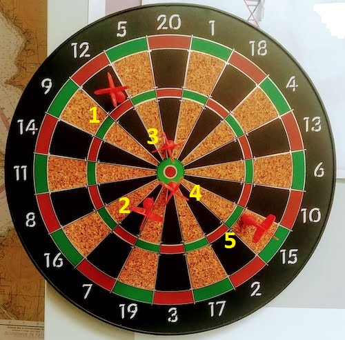
Figure 1. Magnetic dart board with 5 darts. Click image to view full sized image.
The distance in centimeters (cm) between where each of the five darts landed on the board compared to the bullseye is reported in (Table 1),
Table 1. Results of five darts thrown at a target (Figure 2)*
| Dart | Distance |
|---|---|
| 1 | 7.5 |
| 2 | 3.0 |
| 3 | 1.0 |
| 4 | 2.7 |
| 5 | 7.4 |
* distance in centimeters from the center.
Note 1: Use of the coordinate plane, and including the angle measurement in addition to distance (the vector) from center, would be a better analysis. In the context of darts, determining accuracy of a thrower is an Aim-Point targeting problem and part of your calculation would be to get MOA (minute of angle). For the record, the angles (degrees) were
| Dart | Distance | Angle |
|---|---|---|
| 1 | 7.5 | 124.4 |
| 2 | 3.0 | -123.7 |
| 3 | 1.0 | 96.3 |
| 4 | 2.7 | -84.3 |
| 5 | 7.4 | -31.5 |
measured using imageJ. Because there seems to be an R package for just about every data analysis scenario, unsurprisingly, there’s an R package called shotGroups to analyze shooting data.
How precise was the dart thrower? We’ll use the coefficient of variation as a measure of precision. Second, how accurate were the throws? Use R to calculate
darts = c(7.5, 3.0, 1.0, 2.7, 7.4)
#use the coefficient of variation to describe precision of the throws
coefVar = 100*(sd(darts)/mean(darts)); coefVar
[1] 68.46141
Confidence Interval to describe accuracy.
For a game of darts, the true value would be a distance of zero — all bullseyes. We need to calculate the standard error of the mean (SEM), then, we calculate the confidence interval around the sample mean.
#Calculate the SEM
SEM <- sd(darts)/sqrt(length(darts)); SEM
[1] 1.322649
#now, get the lower and upper limit, subtract from the mean
confidence <- c(mean(darts)-2*SEM, mean(darts), mean(darts)+2*SEM); confidence
[1] 1.674702, 4.320000, 6.965298
The mean was 4.3 cm, therefore to get the lower limit of the interval subtract 2.65 (2*SEM = 2.645298) from the mean; for the upper limit add 2.65 to the mean. Thus, we report our approximate confidence interval as (1.7, 7.0), and we read this as saying we are about 95% confident the population value is between these two limits. Five is a very small sample number, so we shouldn’t be surprised to learn that our approximate confidence interval would be less than adequate. In statistical terms, we would use the t-distribution, and not the normal distribution, to make our confidence interval in cases like this.
Note 2: As a rule, implied by Central Limit theory and use of asymptotic statistical estimation, a sample size of 30 or more is safer, but probably unrealistic for many experiments. This is sometimes called as the rule of thirty. (For example, a 96-well PCR array costs about $500; with n = 30, that’s $15,000 US Dollars for one group!). So, what about this rule? This type of thinking should be avoided as “a relic of the pre-computer era,” (Hesterberg, T. (2008). It’s Time To Retire the” n>= 30″ rule.). We can improve on asymptotic statistics by applying bootstrap principles (Chapter 19).
We made a quick calculation of the confidence interval; we can get make this calculation by hand by incorporating the t distribution. We need to know the degrees of freedom, which in this case is 4 (n – 1, where n = 5). We look up critical value of t at 5% (to get our 95% confidence interval), t = 2.78. Subtract for lower limit t*SEM and add for upper limit t*SEM to the sample mean for the 95% confidence interval.
We can get help from R, by using the one-sample t-test with a test against the hypothesis that the true mean is equal to zero. Among a variety of output we will introduce later (see Chapter 8 and 10), the confidence interval is reported (yellow highlight),
#make an attach a data frame object
Ddarts <- data.frame(darts)
t.test(darts,mu=0)
One Sample t-test
data: darts
t = 3.2662, df = 4, p-value = 0.0309
alternative hypothesis: true mean is not equal to 0
95 percent confidence interval:
 0.6477381 7.9922619
sample estimates:
mean of x
 4.32
t.test uses the function qt(), which provides the quantile function. To recreate the 95% CI without the additional baggage output from the t.test, we would simply write
#upper limit
mean(darts)+ qt(0.975,df=4)*sd(darts)/sqrt(5)

#lower limit
mean(darts)+ qt(0.025, df = 4, lower.tail=TRUE)*sd(darts)/sqrt(5)
where sd(darts)/sqrt(5) is the standard error of the mean.
Or, alternatively, download and take advantage of a small package called Rmisc (not to be confused with the RcmdrMisc package) and use the function CI
library(Rmisc)
CI(darts)
     upper     mean     lower
7.9922619 4.3200000 0.6477381
The advantage of using the CI() command from the package Rmisc is pretty clear; I don’t have to specify the degrees of freedom or the standard error of the mean. By default, CI reports the 95% confidence interval. we can specify any interval simply by adding to the command. For example,
CI(darts, ci=0.90)
reports upper and lower limits for the 90% confidence interval.
Try it. On your own, get the 90% confidence interval and the 99% confidence intervals for our dart example. Compare to the 95% confidence interval — what do you conclude about “confidence” in our estimate from 90% to 99%?
Confidence intervals from p-values.
And finally, it is not unusual for a report to provide summary statistics, differences between means (ie, effect size), and p-values (orange highlight), but not report confidence intervals. We discuss p-values and the concept of statistical significance beginning in Chapter 8. But for now, we show how to calculate approximate confidence intervals from the p-value. This may be of use for conducting meta-analysis (Chapter 20.15). See two helpful “how to” articles by Bland and Altman in 2011 BMJ (references listed in Chapter 3.6 – References).
In brief, calculate the test statistic for a normal distribution (letZ), calculate a standard error, and then the lower and upper limits for the 95% confidence interval. We illustrate use of the calculator formulas with the dart example, the p-value was 0.0309; the estimate was 4.32.
R code
letZ = (-0.862 + sqrt(0.743 - 2.404*log(0.0309, base = exp(1)))) = 2.154903
letSE = 4.32/letZ = 2.00473
1.96*letSE = 3.929271 # Add for upper and subtract for lower
The lower limit is 0.39 (4.32 – 3.929271) and the upper limit is 8.25 (4.32 + 3.929271). Although in the ballpark, these calculated estimates are wider than the confidence interval estimated by the t.test command. Small sample size, n = 5, is to blame — the accuracy of these methods, based on asymptotic statistical estimation approaches, assumes the law of large numbers applies.
Significant figures.
And finally, we should respect significant figures, the number of digits which have meaning. Our data were measured to the nearest tenth of a centimeter, or two significant figures. Therefore, if we report the confidence interval as (0.6477381, 7.9922619), then we imply a false level of precision, unless we also report our random sampling error of measurement.
R has a number of ways to manage output. One option would be to set number of figures globally with the options() function — all values reported by R would hold for the entire session. For example, options(digits=3) would report all numbers to three significant figures. Instead, I prefer to use signif() function, which allows us to report just the values we wish and does not change reporting behavior for the entire session.
signif(CI(darts),2)
upper  mean lower
 8.00  4.30  0.65
Note 3: The options() function allows the R user to set a number of settings for an R session. After gaining familiarity with R, the advanced user recognizes that many settings can be changed to make the session work to report in ways more convenient to the user. If curious, submit options() at the R prompt and available settings will be displayed.
The R function signif() applies rounding rules. We apply rounding rules when required to report estimates to appropriate levels of precision. Rounding procedures are used to replace a number with a simplified approximation. Wikipedia provides a comprehensive list of rounding rules. Notable rules include
- directed rounding to an integer, eg, rounding up or down
- rounding to nearest integer, eg, round half up (down) if the number ends with 5
- randomly rounding to an integer, eg, stochastic rounding.
With the exception of stochastic rounding, all rounding methods impose biases on the sets of numbers. For example, the round half up method applied for numbers above 5, round down for numbers below 5 will increase the variance of the sample. In R, use round() for most of your work. If you need one of the other approaches, for example, to round up, the command is ceiling(); to round down we use floor().
When to round?
No doubt your previous math classes have cautioned you about the problems of rounding error and their influence on calculation. So, as a reminder, if reporting calls for rounding, then always round after you’ve completed your calculations, never during the calculations themselves.
A final note about significant figures and rounding. While the recommendations about reporting statistics are easy to come by (and often very proscriptive, eg, Table 1, Cole 2015), there are other concerns. Meta-analysis, which are done by collecting information from multiple studies, would benefit if more and not fewer numbers are reported, for the very same reason that we don’t round during calculations.
Questions
- Calculate the correct 90% and 99% confidence intervals for the dart data using the t-distribution
- by hand
- by one alternative method in R, demonstrated with examples in this page
- How many significant figures should be used for the volumetric pipettor p1000? The p200? The p20 (data at end of this page)?
- Another function,
round(), can be used. Try
round(CI(darts),2)
-
- and report the results: vary the significant figures from 1 to 10 (
signif()will take digits up to 22). - See any output differences between
signif()andround()? Don’t forget to take advantage of R help pages (eg, enter?roundat the R prompt) and see Wikipedia.
- and report the results: vary the significant figures from 1 to 10 (
- Compare rounding by
signif()andround()for the number 0.12345. Can you tell which rounding method the two functions use? - Calculate the coefficient of variation (CV) for each of the three volumetric pipettors from the data at end of this page. Rank the CV from smallest to largest. Which pipettor had the smallest CV and would therefore be judged the most precise?
- (data provided at end of this page, click here).
- Standards distinguish between within run precision and between run precision of a measurement instrument (see Chapter 16.5 – Instrument reliability and validity). The data in Table 1 were all recorded within 15 minutes by one operator. What kind pf precision was measured?
- Calculate the standard error of the means for each of the three pipettors from the data
- (data provided at end of this page, click here).
- Calculate the approximate confidence interval using the 2SE rule and judge which of the three pipettors is the most accurate (narrowest confidence interval)
- Repeat, but this time apply your preferred R method for obtaining confidence intervals.
- Compare approximate and R method confidence intervals. How well did the approximate method work?
- Return to the dart example, but now assume the p-value was p = 0.003 and again for p = 0.0003. Estimate the 95% confidence interval for each case; the difference remains 4.32. How does the change in p-value, from 0.03 to 0.0003 — a two orders of magnitude difference — affect the estimates for the confidence interval (hint: describe the width of the CI)?
Quiz Chapter 3.5
Statistics of error
Data sets
Pipette calibration
| p1000 | p200 | p100 |
|---|---|---|
| 0.113 | 0.1 | 0.101 |
| 0.114 | 0.1 | 0.1 |
| 0.113 | 0.1 | 0.1 |
| 0.115 | 0.099 | 0.101 |
| 0.113 | 0.1 | 0.101 |
| 0.112 | 0.1 | 0.1 |
| 0.113 | 0.1 | 0.1 |
| 0.111 | 0.1 | 0.1 |
| 0.114 | 0.101 | 0.101 |
| 0.112 | 0.1 | 0.1 |
Chapter 3 continues
6.1 – Some preliminaries
Introduction
OK, you say, I get it: statistics is important, and if I am to go on as a biologist, I should learn statistics. Let’s get on with it, start with the equations and the problems already!
Before we review probability theory and introduce risk analysis I want to spend some time to emphasize that at issue is critical thinking, so please bear with me (Fig 1).
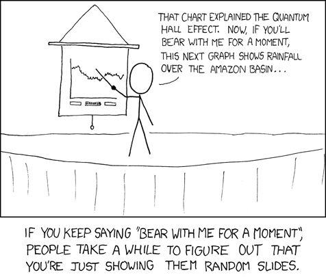
Figure 1. “Slides,” https://xkcd.com/365/.
How likely?
As we start our journey in earnest, we start with the foundations of statistics, probability. Probability in statistics means the chance that a specific outcome will occur. Probability is something we measure, or estimate, or draw from theoretical models, about whether something, a specific outcome from a class of outcomes (events — see Chapter 7.1), will occur. We speak about how likely an outcome is to occur, and this is quantified by the probability. Probabilities are given a value between 0 and 1: at 0% chance, the event will not happen; 100% chance, the event is certain to happen. Remember, probability applies to predicting future events; obviously, when viewed in the past, the event either did (100%), or did not (0%) happen.
If probability is the chance that an outcome will occur, then risk is the probability of a particular outcome occurring over a specified period of time. Related, epidemiologists define exposure risk as the potential for harm (or benefit) from contact with or vulnerability to a hazard (or treatment) or risk factor.
I introduce our discussion of probability through a risk analysis — the process of evaluating the probability and potential impact of health risks to individuals or populations. I like to start this discussion by relaying something I overheard while a number of us were standing on a lava field on the slopes of Kilauea back in November of 1998 (Kilauea erupted with lava flow more or less continually between 1983 and 2018; 5 Jan 2023, started up again).

Figure 2. View of Kamokuna Lava Bench, eruption of Pu`u `O`o, Kilauea, November 1998. Photo by S. Dohm.
In 1998, Volcanoes National Park hadn’t established barricades at the end of Chain of Craters Road, and people were walking to see new lava flows. The night we went, we met a park ranger who pleaded with us that the Park Service believed it was unsafe for us to walk out to see new lava flows because the area, called a lava delta, was unstable. Someone (not in my group), snapped back, “Oh, what are the chances that that will happen?” Of course, the ranger couldn’t quote a chance between zero and 100% for that particular evening. The ranger was saying the risk had increased, based on their subjective, but experienced opinion (see Kinds of probability, below).
As you can see in Figure 2, we went anyway. I have been thinking about her question ever since. We were lucky — some of the same area collapsed two weeks later (SOEST information, eruption about episode 55).
Cool picture though.
While the terms are used interchangeably in everyday language, they have distinct mathematical and statistical definitions. Prospective: You use a known model and its parameters to predict the probability of future data.
Multiple events
Whether or not a newly formed lava delta collapses, that’s a singular or simple event. For cases with more than one one outcome, that’s a multiple event.
I have two coins, a dime and a quarter, in my pocket; when I place the coins on the table, what are the chances that both coins will show heads? A blood sample from a crime scene was typed for two Combined DNA Index System (CODIS) Short Tandem Repeat (STR) loci, THO1 (allele 9.3) and TPOX (allele 8), the same allele types for the defendant. What are the chances of a match, someone other than the defendant has the same genetic profile? In both examples I describe a random process. With randomness, we can predict the probability of each kind of outcome, or series of outcomes, because we know the total possible number of outcomes. If there are just two outcomes, then the probability is equal — 50% that either will occur. If, however, the process is not random, then even if there are just two possible outcomes, the probability can’t be 50% — the outcome depends on some other process than random chance.
What is the chance that two events occur? For two or more independent events we can get the answers by using the product rule.

The two coins are independent, therefore the chance that both are placed heads up is 25% — we would expect to see this combined event one out of every four times. This is an illustration of the counting rule, aka fundamental counting principle: if there are n ways to do one thing (n elements in set A), and m ways to do another thing (m elements in set B), then there are  ways to do both things (combination of elements of A and B sets).
For the DNA profile CODIS problem (cf. Chapter 4, National Research Council 1996), the two alleles are both the most common observed in US Caucasian population at 30.45% and 54.7%, respectively (Moretti et al 2016). Assuming the individual was homozygous at both loci (ie, THO19.3,9.3 and TPOX8,8), then the genotype frequencies (p2) are:


Since THO1 is located on the p arm of chromosome 11, and TPOX is on the p arm of chromosome 2, the two loci are independent and therefore should be in linkage disequilibrium. We can use the product rule to get the probability of the DNA profile for the sample, 2.8%

If two events are not independent, then the product rule cannot be used. For example, CODIS STR D5S818 and CSF1PO are both located on the q arm of chromosome 5 and are therefore linked and not independent (the recombination frequency is about 0.25). The common allele for D5S818 is 11 at 40.84% and for CSF1PO the allele is 12 at 34.16%. Thus the chance that the two most common alleles is not simply the product rule result of 14%, instead we need to view this problem as one of dependent events.
Kinds of probability.
So, how does one go about estimating the likelihood that a particular event, whether it is collapse of a lava delta, or that a person will have a heart attack? The probability of lava delta collapse or of heart attack are examples of empirical probability, as opposed to a theoretical probability. Despite many years of effort, we have no applicable theory that we can apply to say, if a person does this, and that, then a heart attack will happen. But we do have a body of work documenting how often heart attacks occur, and when they occur in association with certain risk factors. Similarly, progress is being made to determine markers of risk of lava field collapse (Di Traglia et al. 2018). Analogously, this is the essential goal of risk analysis in epidemiology. We know of associations between cholesterol and heart attack risk, for example, but we also know that high cholesterol does not raise the probability of the event (heart attack) to 100%. How is this uncertainty part of statistics? Or perhaps you are a molecular scientist in training and have learned about how to assess results of a Western blot where typically the results are scored as “yes” or “no.” How is this relevant to statistics and probability?
A misconception about statistics and statistical thinking
There’s a long history of skepticism of conclusions from health studies, in part because it seems the advice flips. For example,
- Coffee is bad for you (Medical News Today January 2008)
- Coffee is good for you (NBC News July 2018)
- Even light drinking can be harmful to health (Science Daily, January 2022)
- Seven science-backed reasons beer is good for you (NBC News August 2017)
- Meat and cheese may be as bad for you as smoking (Science Daily, March 2014)
- Cheese actually isn’t bad for you (WIRED, February 2021)
The common thread is these studies are assessment of risk: about studies that seem to conclude “only: with statements of probability.
Perhaps you may have heard …? “There are lies and then there is statistics“. The full quote reads as follows:
Figures often beguile me, particularly when I have the arranging of them myself; in which case the remark attributed to Disraeli would often apply with justice and force: “There are three kinds of lies: lies, damned lies and statistics.” – Autobiography of Mark Twain (www.twainquotes.com/Lies.html).
Figure 3. Mark Twain. Image from The Miriam and Ira D. Wallach Division of Art, Prints and Photographs: Photography Collection, The New York Public Library. “Mark Twain in Middle Life” The New York Public Library Digital Collections. 1860 – 1920. https://digitalcollections.nypl.org/items/510d47d9-baec-a3d9-e040-e00a18064a99
Twain attributed the remarks to Benjamin Disraeli, the prime minister of Britain during much of Queen Victoria’s reign, but others have not been able to document this utterance to that effect. Still others believe that the “3-lies” quote belongs to Leonard Courtney, an English mathematician and statistician (1847-1929) (see University of York web site for more).
What is meant by this quote? Tossing aside cynicism — or healthy skepticism of authority one should have, whether that authority is a scientist or a politician(within reason, please!) — what this quote means is that it seems that results of very similar studies are in conflict. To some, this is part of the replication crisis in science (Baker 2016). There’s a perception that one can say just about anything with a number. Partly this is a matter of semantics, but also there is legitimacy to this concern. However, it is not necessarily the case that statistics have been intentionally done to mislead, rather, there is evidence that researchers are not always using proper statistical procedures.
One word, several meanings
We use the term statistics in multiple ways, all correct, but not all equal. For example, a statistic may refer to a number used to describe a population characteristic. From the 2010 U.S. census, we learn that the racial (self-reported) make-up of the U.S. population (then at 303 million) was 72.4% “white” and 12.6% “black” self-reported. In this sense, a statistic is something you calculate as a description. Do you recall the distinction between “statistic” and “statistics” discussed in Chapter 2?
Secondly, two studies essentially about the same topic, yet reaching seemingly different conclusions, may differ in the assumptions employed. It should be obvious that if different assumptions are used, researchers may reach different outcomes.
Finally, how we communicate statistics can be misleading. For example, use of percentages in particular can be confusing, especially in communication of the chance that some event may happen to us (eg, incidence of disease: number of new cases in a specific time period, compared to prevalence of a disease: number of cases of a disease in a specific period of time). On the one hand, percentages seem easy. A percentage is simply a proportion multiplied by 100%, and takes any value between 0% and 100%.
When a product says that it kills 99.99% of all germs on contact, do you feel better? Here’s a cartoon to consider as you think about that statement (Fig 4).
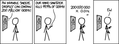
Figure 4. “Hand sanitizer,” https://imgs.xkcd.com/comics/hand_sanitizer.png
Of course numbers cannot be used to justify simultaneously mutually exclusive conclusions, but being able to recognize careless (or deliberate) miscommunication with numbers, well, this needs to be part of your skill set. Here’s a little exercise from transportation safety to ponder as you reflect on the subject of lies and statistics. rather, as you read this next section I ask that you consider
- are the correct statistical descriptors in use?
- what assumptions are being made?
- does the reporting of percentages lead to clear conclusions?
Some concluding thoughts about “lies and statistics”
Statistics is tricky because there are assumptions to be made. And you have to be clear in your thinking.
If the assumptions hold true, then we aren’t lying, and Twain had it wrong.
But if we disagree on the assumptions, then we will necessarily have to disagree on the conclusions drawn from the calculated numbers (the statistics). Risk analysis in particular, but statistics in general, is a tricky business because many assumptions need to be made, and we won’t necessarily have all of the relevant information available to make sure our assumptions are truthful. But it is the assumptions that matter: if we agree with the assumptions that are made, then we have confidence in the conclusions drawn from the statistics.
In a typical statistics course, we would spend a bunch of time on probability. We will here as well, but in the context of risk analysis and in the other contexts, in a less than formal presentation on the subject of probability. For example, in talking about inference, the testing of null hypotheses and estimating the probability that the null hypothesis is correct, I will say things like, “Imagine we repeated the experiment a million times — how many times by chance would we think a correct null hypothesis would none the less be rejected?”
There’s no real substitute for a formal course in probability theory and you should be aware that this foundation is pretty important if you go forward with biostatistics and epidemiology. For now, I will simply refer you to chapters 1, 2 and 3 of a really nice online book on probability from one of the masters, Richard Jeffrey (1926 – 2002; click here to go to Wikipedia). Much of what I will present to you follows from similar discussions.
My aim is to teach you what you need about probability theory by the doing. In the next couple of days we will deal with an aspect of risk analysis, namely a consideration of conditional probability and Baye’s Theorem that will help you evaluate claims such as the one made for airline safety. Risk analysis is tricky, but it is not a subject above and beyond our abilities; by applying some of the rules of statistical reasoning, we can check claims based on statistics. A healthy degree of skepticism is part of becoming a scientist. Do try this at home!
Some examples to consider: what is the relative risk for the following scenarios?
1. Drug testing at the workplace: risk of a worker, who does not use illegal drugs, registering positive (false positives in drug testing);
2. Positive HIV from blood sample from USA male with no associated risks (eg, intravenous drug user), false positives in HIV testing; false positives with mammography;
3. Benefits versus risks of taking a statin drug (drug that reduces serum cholesterol levels) to a person with no history of heart disease.
4. Is it safer to travel by car or by airliner? We’ll break this problem down in the next section.
What we are looking for is the probability of an occurrence of a particular event: that a person who does not use illegal drugs may nonetheless test positive; we are looking for a way to make rational decisions and understanding probability is the foundation.
Questions
- What do you make of the claim (joke) that “There are lies and then there are statistics?”
- Distinguish between empirical and theoretical probability; use examples.
Quiz Chapter 6.1
Some preliminaries
Chapter 6 contents
- Introduction
- Some preliminaries
- Ratios and proportions
- Combinations and permutations
- Types of probability
- Discrete probability distributions
- Continuous distributions
- Normal distribution and the normal deviate (Z)
- Moments
- Chi-square distribution
- t distribution
- F distribution
- References and suggested readings
6 – Probability, Distributions
Introduction
Probability is how likely something, an event, is likely to occur, ie, a prediction of the future. Related, we can ask of the likelihood of an event, which is like working backwards. The event has already occurred and we ask how well a model (parameters) explain the observed data.
Working with probability allows us to contextualize the inherent uncertainty in any measure, which in turn allows us to interpret results from hypothesis tests of observational or experimental data sets. Thus, an important concept to appreciate is that in many cases, like R.A. Fisher’s Lady tasting tea analogy, we can count in advance all possible outcomes of an experiment.
For many more experiments, we cannot count all possible outcomes of the sample space, either because they are too numerous or simply unknowable. In such cases, applying theoretical probability distributions allow us to circumvent the countability problem. Whereas empirical probability distributions are frequency counts of observations, theoretical probabilities are based on mathematical formulas.
At this stage of your training in statistics, you would spend time with the foundations of probability. Scenarios of likelihood of single events regardless of other events are called marginal probability, whereas the union refers to at least one event occuring. The likelihood of two or more events occuring at the same time is called joint probability. Worked examples are presented in the chapter, although the bulk of this chapter concerns conditonal probability, the likelihood of one event occuring given another event already happened. Working with conditional probability is essential for risk analysis, which we introduce in Chapter 7 – Probability, Risk Analysis and expand in Chapter 7.3 – Conditional Probability and Evidence Based Medicine and Chapter 7.4 – Epidemiology: Relative risk and absolute risk, explained.
Probability distributions are key to the null hypothesis significance testing framework for statistical inference. Given assumptions about the data, probability distributions are used to evaluate the likelihood of observing data under the null hypothesis, eg, no difference between means of a control group compared to a treatment group. Much of classical inferential statistics, especially the kind one finds in introductory courses like ours, are built on probability distributions. ANOVA, t-tests, linear regression, etc., are parametric tests and assume errors are distributed according to a particular type of distribution, the normal or Gaussian distribution.
A probability distribution is a list of probabilities for each possible outcome of a discrete random variable in an entire population. Depending on the data type, there are many classes of probability distributions. In contrast, probability density functions are used to for continuous random variables. This chapter begins with basics of probability then gently introduces discrete and continuous probability distributions. In the other sections of this chapter we describe several probability density functions. Emphasis is placed on the normal distribution, which underlies most parametric statistics.
Homework to go with this topic
Homework 3: Distributions & Probability in Mike’s Workbook for Biostatistics.
Quizzes in this chapter
A total of 88 questions among the several subchapters, a mix of true or false and multiple choice question format.
Chapter 6 contents
- Introduction
- Some preliminaries
- Ratios and proportions
- Combinations and permutations
- Types of probability
- Discrete probability distributions
- Continuous distributions
- Normal distribution and the normal deviate (Z)
- Moments
- Chi-square distribution
- t distribution
- The F distribution
- References and suggested readings