3.5 – Statistics of error
Making sense of error in data.
This page explains how statistics of error help quantify differences between measured and true values, beginning with classical methods like standard error and confidence intervals that rely on large-sample assumptions. Related, statisticians talk about uncertainty — the quantification of doubt about a measurement. We introduce permutation-based approaches, including jackknife and bootstrap resampling, which avoid those assumptions and are especially useful with smaller or complex data sets. Observer variation (intra- and interobserver error) is also highlighted as an important source of measurement error.
Missing values are another common source of uncertainty in biological data sets. Data may be missing because of equipment failure, recording mistakes, sample loss, or biological factors that prevent a measurement from being collected. Even a small number of missing observations can influence summaries, graphs, and statistical tests, especially in smaller studies. In this chapter, we treat missing values mainly as a practical issue to identify and report during exploratory data analysis. Later, in the chapter on experimental design, we examine missing data in greater depth, including differences between random and non-random missingness, as well as approaches such as data imputation and the consequences these choices may have for interpretation.
We conclude with a discussion about confidence intervals as a measure of accuracy and emphasize proper use of significant figures to avoid overstating precision.
Statistics of error.
In statistics, error doesn’t mean mistake, an avoidable human misjudgement or oversight, eg, a typo. An error in statistics means there was a difference between the measured value and the actual value for an object. Efforts by many authors of notable classical statistics developed a large body of calculated statistics, eg, standard error the mean, which allows the user to quantify how large the error of measurement is given assumptions about the distribution of the errors. Thus, classical statistics requires user to make assumptions about the error distribution, the subject of our Chapter 6. A critical issue to understand is that these methods assume large sample sizes are available; they are called asymptotic statistics or large-sample statistics; the properties of the statistical estimates are evaluated as sample size approaches infinity.
Jackknife sampling and bootstrap sampling are permutation approaches to working with data when the Central Limit Theorem — as sample size increases, the distribution of sample means will tend to a normal distribution (see Chapter 6.7) — is unlikely to apply or, rather, we don’t wish to make that assumption (Chapter 19). The jackknife is a sampling method involving repeatedly sampling from the original data set, but each time leaving one value out. The estimator, for example, the sample mean, is calculated for each sample. The repeated estimates from the jackknife approach yield many estimates which, collected, are used to calculate the sample variance. Jackknife estimators tend to be less biased than those from classical asymptotic statistics.
Bootstrapping, and not jackknife resampling, may now be the preferred permutation approach (eg, Google Scholar search “bootstrap statistics” 36K hits; “jackknife statistics” 17K hits), but which method is best depends on qualities of the data set. Bootstrapping involves large numbers of permutations of the original data, which, in short, means we repeatedly take many samples of our data and recalculate our statistics on these sets of sampled data. We obtain statistical significance by comparing our result from the original data against how often results from our permutations on the resampled data sets exceed the originally observed results. By permutation methods, the goal is to avoid the assumptions made by large-sample statistical inference, ie, reaching conclusions about the population based on samples from the population. Since its introduction, “bootstrapping” has been shown to be superior in many — but, importantly, not all — cases for statistics of error compared to the standard, classical approach (Efron 1979, Hesterberg 2015).
There are many advocates for the permutation approaches, and, because we have computers now instead of the hand calculators our statistics ancestors used, permutation methods may be the approach you will take in your own work. However, the classical approach has its strengths — when the conditions, that is, when the assumptions of asymptotic statistics are met by the data, then the classical approaches tend to be less conservative than the permutation methods. By conservative, statisticians mean that a test performs at the level we expect it to. Thus, if the assumptions of classical statistics are met they return the correct answer more often than do the permutation tests.
Error and the observer.
Individual researchers make observations, therefore, we can talk about observer variation as a kind of error measurement. For repeated measures of the same object by an individual, we would expect the individual to return the same results. To the extent repeated measures differ, this is intraobserver error. In contrast, measures of the same object from different individuals is interobserver error. For a new instrument or measurement system, one would need to establish the reliability of the measure: confronted with the same object do researchers get the same measurement? Accounting for interobserver error applies in many fields, eg, histopathology of putative carcinoma slides (Franc et al 2003), liver biopsies for cirrhosis (Rousselet et al 2005), blood cell counts (Bacus 1973).
Confidence in estimates.
A really useful concept in statistics is the idea that you can assign how confident you are to an estimate. This is another way to speak of the accuracy of an estimate. Clearly, we have more confidence in a sample estimate for a population parameter if many observations are made. Another factor in our ability to estimate is the magnitude of observation differences. In general, the larger the differences among values from repeated trials, the less confident we will be in out estimate, unless, again, we make our estimates from a large collection of observations. These two quantities, sample size and variability, along with our level of confidence, eg, 95%, are incorporated into a statistic called the confidence interval.

We will use this concept a lot throughout the course; for now, a simple but approximate confidence interval is to use the 2 x SEM rule (as long as sample size large): twice the standard error of the mean. Take your estimate of the mean, then add (upper limit) or subtract (lower limit) twice the value of the standard error of the mean (if you recall, that’s the standard deviation divided by the square-root of the sample size).
Example. Consider five magnetic darts thrown at a dart board (28 cm diameter, height of 1.68m from the floor) from a distance of 3.15 meters (Fig 1).
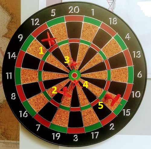
Figure 1. Magnetic dart board with 5 darts. Click image to view full sized image.
The distance in centimeters (cm) between where each of the five darts landed on the board compared to the bullseye is reported in (Table 1),
Table 1. Results of five darts thrown at a target (Figure 2)*
| Dart | Distance |
|---|---|
| 1 | 7.5 |
| 2 | 3.0 |
| 3 | 1.0 |
| 4 | 2.7 |
| 5 | 7.4 |
* distance in centimeters from the center.
Note 1: Use of the coordinate plane, and including the angle measurement in addition to distance (the vector) from center, would be a better analysis. In the context of darts, determining accuracy of a thrower is an Aim-Point targeting problem and part of your calculation would be to get MOA (minute of angle). For the record, the angles (degrees) were
| Dart | Distance | Angle |
|---|---|---|
| 1 | 7.5 | 124.4 |
| 2 | 3.0 | -123.7 |
| 3 | 1.0 | 96.3 |
| 4 | 2.7 | -84.3 |
| 5 | 7.4 | -31.5 |
measured using imageJ. Because there seems to be an R package for just about every data analysis scenario, unsurprisingly, there’s an R package called shotGroups to analyze shooting data.
How precise was the dart thrower? We’ll use the coefficient of variation as a measure of precision. Second, how accurate were the throws? Use R to calculate
darts = c(7.5, 3.0, 1.0, 2.7, 7.4)
#use the coefficient of variation to describe precision of the throws
coefVar = 100*(sd(darts)/mean(darts)); coefVar
[1] 68.46141
Confidence Interval to describe accuracy.
For a game of darts, the true value would be a distance of zero — all bullseyes. We need to calculate the standard error of the mean (SEM), then, we calculate the confidence interval around the sample mean.
#Calculate the SEM
SEM <- sd(darts)/sqrt(length(darts)); SEM
[1] 1.322649
#now, get the lower and upper limit, subtract from the mean
confidence <- c(mean(darts)-2*SEM, mean(darts), mean(darts)+2*SEM); confidence
[1] 1.674702, 4.320000, 6.965298
The mean was 4.3 cm, therefore to get the lower limit of the interval subtract 2.65 (2*SEM = 2.645298) from the mean; for the upper limit add 2.65 to the mean. Thus, we report our approximate confidence interval as (1.7, 7.0), and we read this as saying we are about 95% confident the population value is between these two limits. Five is a very small sample number, so we shouldn’t be surprised to learn that our approximate confidence interval would be less than adequate. In statistical terms, we would use the t-distribution, and not the normal distribution, to make our confidence interval in cases like this.
Note 2: As a rule, implied by Central Limit theory and use of asymptotic statistical estimation, a sample size of 30 or more is safer, but probably unrealistic for many experiments. This is sometimes called as the rule of thirty. (For example, a 96-well PCR array costs about $500; with n = 30, that’s $15,000 US Dollars for one group!). So, what about this rule? This type of thinking should be avoided as “a relic of the pre-computer era,” (Hesterberg, T. (2008). It’s Time To Retire the” n>= 30″ rule.). We can improve on asymptotic statistics by applying bootstrap principles (Chapter 19).
We made a quick calculation of the confidence interval; we can get make this calculation by hand by incorporating the t distribution. We need to know the degrees of freedom, which in this case is 4 (n – 1, where n = 5). We look up critical value of t at 5% (to get our 95% confidence interval), t = 2.78. Subtract for lower limit t*SEM and add for upper limit t*SEM to the sample mean for the 95% confidence interval.
We can get help from R, by using the one-sample t-test with a test against the hypothesis that the true mean is equal to zero. Among a variety of output we will introduce later (see Chapter 8 and 10), the confidence interval is reported (yellow highlight),
#make an attach a data frame object
Ddarts <- data.frame(darts)
t.test(darts,mu=0)
One Sample t-test
data: darts
t = 3.2662, df = 4, p-value = 0.0309
alternative hypothesis: true mean is not equal to 0
95 percent confidence interval:
 0.6477381 7.9922619
sample estimates:
mean of x
 4.32
t.test uses the function qt(), which provides the quantile function. To recreate the 95% CI without the additional baggage output from the t.test, we would simply write
#upper limit
mean(darts)+ qt(0.975,df=4)*sd(darts)/sqrt(5)

#lower limit
mean(darts)+ qt(0.025, df = 4, lower.tail=TRUE)*sd(darts)/sqrt(5)
where sd(darts)/sqrt(5) is the standard error of the mean.
Or, alternatively, download and take advantage of a small package called Rmisc (not to be confused with the RcmdrMisc package) and use the function CI
library(Rmisc)
CI(darts)
     upper     mean     lower
7.9922619 4.3200000 0.6477381
The advantage of using the CI() command from the package Rmisc is pretty clear; I don’t have to specify the degrees of freedom or the standard error of the mean. By default, CI reports the 95% confidence interval. we can specify any interval simply by adding to the command. For example,
CI(darts, ci=0.90)
reports upper and lower limits for the 90% confidence interval.
Try it. On your own, get the 90% confidence interval and the 99% confidence intervals for our dart example. Compare to the 95% confidence interval — what do you conclude about “confidence” in our estimate from 90% to 99%?
Confidence intervals from p-values.
And finally, it is not unusual for a report to provide summary statistics, differences between means (ie, effect size), and p-values (orange highlight), but not report confidence intervals. We discuss p-values and the concept of statistical significance beginning in Chapter 8. But for now, we show how to calculate approximate confidence intervals from the p-value. This may be of use for conducting meta-analysis (Chapter 20.15). See two helpful “how to” articles by Bland and Altman in 2011 BMJ (references listed in Chapter 3.6 – References).
In brief, calculate the test statistic for a normal distribution (letZ), calculate a standard error, and then the lower and upper limits for the 95% confidence interval. We illustrate use of the calculator formulas with the dart example, the p-value was 0.0309; the estimate was 4.32.
R code
letZ = (-0.862 + sqrt(0.743 - 2.404*log(0.0309, base = exp(1)))) = 2.154903
letSE = 4.32/letZ = 2.00473
1.96*letSE = 3.929271 # Add for upper and subtract for lower
The lower limit is 0.39 (4.32 – 3.929271) and the upper limit is 8.25 (4.32 + 3.929271). Although in the ballpark, these calculated estimates are wider than the confidence interval estimated by the t.test command. Small sample size, n = 5, is to blame — the accuracy of these methods, based on asymptotic statistical estimation approaches, assumes the law of large numbers applies.
Significant figures.
And finally, we should respect significant figures, the number of digits which have meaning. Our data were measured to the nearest tenth of a centimeter, or two significant figures. Therefore, if we report the confidence interval as (0.6477381, 7.9922619), then we imply a false level of precision, unless we also report our random sampling error of measurement.
R has a number of ways to manage output. One option would be to set number of figures globally with the options() function — all values reported by R would hold for the entire session. For example, options(digits=3) would report all numbers to three significant figures. Instead, I prefer to use signif() function, which allows us to report just the values we wish and does not change reporting behavior for the entire session.
signif(CI(darts),2)
upper  mean lower
 8.00  4.30  0.65
Note 3: The options() function allows the R user to set a number of settings for an R session. After gaining familiarity with R, the advanced user recognizes that many settings can be changed to make the session work to report in ways more convenient to the user. If curious, submit options() at the R prompt and available settings will be displayed.
The R function signif() applies rounding rules. We apply rounding rules when required to report estimates to appropriate levels of precision. Rounding procedures are used to replace a number with a simplified approximation. Wikipedia provides a comprehensive list of rounding rules. Notable rules include
- directed rounding to an integer, eg, rounding up or down
- rounding to nearest integer, eg, round half up (down) if the number ends with 5
- randomly rounding to an integer, eg, stochastic rounding.
With the exception of stochastic rounding, all rounding methods impose biases on the sets of numbers. For example, the round half up method applied for numbers above 5, round down for numbers below 5 will increase the variance of the sample. In R, use round() for most of your work. If you need one of the other approaches, for example, to round up, the command is ceiling(); to round down we use floor().
When to round?
No doubt your previous math classes have cautioned you about the problems of rounding error and their influence on calculation. So, as a reminder, if reporting calls for rounding, then always round after you’ve completed your calculations, never during the calculations themselves.
A final note about significant figures and rounding. While the recommendations about reporting statistics are easy to come by (and often very proscriptive, eg, Table 1, Cole 2015), there are other concerns. Meta-analysis, which are done by collecting information from multiple studies, would benefit if more and not fewer numbers are reported, for the very same reason that we don’t round during calculations.
Questions
- Calculate the correct 90% and 99% confidence intervals for the dart data using the t-distribution
- by hand
- by one alternative method in R, demonstrated with examples in this page
- How many significant figures should be used for the volumetric pipettor p1000? The p200? The p20 (data at end of this page)?
- Another function,
round(), can be used. Try
round(CI(darts),2)
-
- and report the results: vary the significant figures from 1 to 10 (
signif()will take digits up to 22). - See any output differences between
signif()andround()? Don’t forget to take advantage of R help pages (eg, enter?roundat the R prompt) and see Wikipedia.
- and report the results: vary the significant figures from 1 to 10 (
- Compare rounding by
signif()andround()for the number 0.12345. Can you tell which rounding method the two functions use? - Calculate the coefficient of variation (CV) for each of the three volumetric pipettors from the data at end of this page. Rank the CV from smallest to largest. Which pipettor had the smallest CV and would therefore be judged the most precise?
- (data provided at end of this page, click here).
- Standards distinguish between within run precision and between run precision of a measurement instrument (see Chapter 16.5 – Instrument reliability and validity). The data in Table 1 were all recorded within 15 minutes by one operator. What kind pf precision was measured?
- Calculate the standard error of the means for each of the three pipettors from the data
- (data provided at end of this page, click here).
- Calculate the approximate confidence interval using the 2SE rule and judge which of the three pipettors is the most accurate (narrowest confidence interval)
- Repeat, but this time apply your preferred R method for obtaining confidence intervals.
- Compare approximate and R method confidence intervals. How well did the approximate method work?
- Return to the dart example, but now assume the p-value was p = 0.003 and again for p = 0.0003. Estimate the 95% confidence interval for each case; the difference remains 4.32. How does the change in p-value, from 0.03 to 0.0003 — a two orders of magnitude difference — affect the estimates for the confidence interval (hint: describe the width of the CI)?
Quiz Chapter 3.5
Statistics of error
Data sets
Pipette calibration
| p1000 | p200 | p100 |
|---|---|---|
| 0.113 | 0.1 | 0.101 |
| 0.114 | 0.1 | 0.1 |
| 0.113 | 0.1 | 0.1 |
| 0.115 | 0.099 | 0.101 |
| 0.113 | 0.1 | 0.101 |
| 0.112 | 0.1 | 0.1 |
| 0.113 | 0.1 | 0.1 |
| 0.111 | 0.1 | 0.1 |
| 0.114 | 0.101 | 0.101 |
| 0.112 | 0.1 | 0.1 |
Chapter 3 continues
17.6 – ANCOVA – analysis of covariance
Introduction
Analysis of covariance (ANCOVA) is intended to help with analysis of designs with categorical treatment variables on some response (dependent) variable, but a known confounding variable is also present. Thus, the researcher is also likely to know of additional ratio scale variables that covary with the response variable and, moreover, must be included in the experimental design in some way.
Take for example the well-known relationship between body size and whole-animal metabolic rate as measured by rates of carbon dioxide production or rates of oxygen consumption for aerobic organisms. We may be interested in how addition or blocking of stress hormones affects resting metabolism; we may be interested in comparing men and women for activity metabolism, and so on. We’d like to know if the regressions were the same (eg, metabolic rate covaried with body mass in the same way — that is, the slope of the relationship was the same).
This situation arises frequently in biology. For example, we might want to know if male and female birds have different mean field metabolic rates, in which case we might be tempted to use a one-way ANOVA or t-test (since one factor with two levels). However, if males and females also differ for body size, then any differences we might see in metabolic rate could be due to differences in metabolic rate are confounded by differences in the covariable body size. We already discussed one approach to correction: calculate a ratio. Thus, a logical approach to correcting or normalizing for the covariation would be to divide body mass (units of kilograms) into metabolic rate (eg, volume of oxygen, O2, consumed), and make comparisons, say, among different species, on mass-specific trait ( ). However, because the regression between mass and metabolic rate is allometric, i.e., not equal to one, the ratio does not, in fact normalize for body mass. We made this point in Chapter 6.2, and remarked that analysis of covariance ANCOVA was a solution.
ANCOVA allows you to test for mean differences in traits like metabolic rate between two or more groups, but only after first accounting for covariation due to another variable (eg, body size). However, ANCOVA makes the assumption that relationship between the covariable and the response variable is the same in the two groups. This is the same as saying that the regression slopes are the same. We discussed how to use t-test to test hypothesis of equal slopes between regression models in Chapter 17.5, but a more elegant way is to include this in your model.
Example
We return to our sample of 13 tadpoles (Rana pipiens), hatched in the laboratory. I’ve repeated the data set in this page, scroll or click here.
Our linear model was  and a scatterplot of the data set is shown in Figure 1 (a repeat of Figure 3 from Chapter 17.5, but now points identified to developmental group).
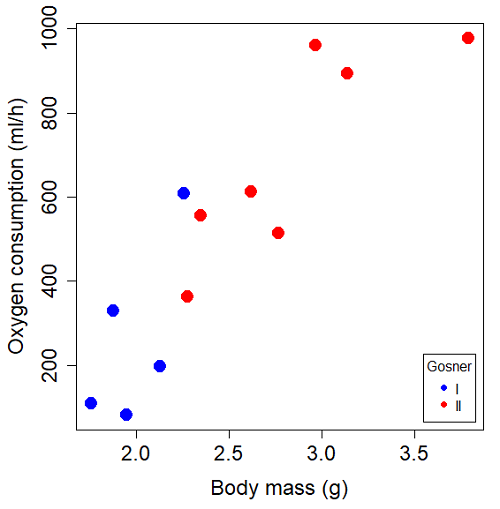
Figure 1. Scatterplot of oxygen consumption by R. pipiens tadpoles vs body mass (g) by developmental group (Gosner stages I or II).
The project looked at whether metabolism as measured by oxygen consumption was consistent across two developmental stages. Metamorphosis in frogs and other amphibians represents profound reorganization of the organism as the tadpole moves from water to air. Thus, we would predict some cost as evidenced by change in metabolism associated with later stages of development. Figure 2 shows a box plot of tadpole oxygen consumption by Gosner (1960) developmental stage (Figure 2 is a repeat of Figure 4 Chapter 17.5).
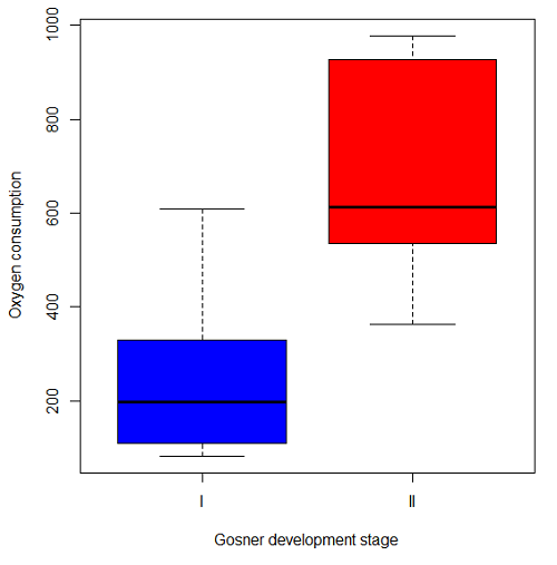
Figure 2. Copy of Figure 4, Chapter 17.5; boxplot of oxygen consumption of R. pipiens tadpoles by Gosner developmental stages.
Looking at Figure 2 we see a trend consistent with our prediction; developmental stage may be associated with increased metabolism. However, older tadpoles also tend to be larger, and the plot in Figure 2 does not account for that. Thus, body mass is a confounding variable in this example. There are several options for analysis here (eg, ANCOVA), but one way to view this is to compare the slopes for the two developmental stages. While this test does not compare the means, it does ask a related question: is there evidence of change in rate of oxygen consumption relative to body size between the two developmental stages? The assumption that the slopes are equal is a necessary step for conducting the ANCOVA.
So, divide the data set (Table 1) into two groups by developmental stage (12 tadpoles could be assigned to one of two developmental stages; one was at a lower Gosner stage than the others and so is dropped from the subset.
Table 1.  and
 of 12 R. pipiens tadpole larvae by Gosner developmental stage.
Gosner stage I
|
|
| 1.76 | 109.41 |
| 1.88 | 329.06 |
| 1.95 | 82.35 |
| 2.13 | 198 |
| 2.26 | 607.7 |
Gosner stage II
| Body mass | |
| 2.28 | 362.71 |
| 2.35 | 556.6 |
| 2.62 | 612.93 |
| 2.77 | 514.02 |
| 2.97 | 961.01 |
| 3.14 | 892.41 |
| 3.79 | 976.97 |
The slopes and standard errors we obtained in Chapter 17.5 were
| Gosner Stage I | Gosner stage II | |
| slope | 750.0 | 399.9 |
| standard error of slope | 444.6 | 111.2 |
Make a plot (Figure 3).
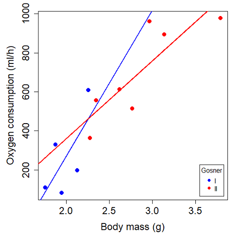
Figure 3. Scatterplot with best-fit regression lines of by for Gosner State I (closed circle, solid line) and Gosner Stage II (open circle, dashed line) R. pipiens tadpoles.
R code for plot in Figure 3.
#Used Rcmdr scatterplot(), then modified code
scatterplot(VO2~Body.mass | Gosner, regLine=FALSE, smooth=FALSE,
boxplots=FALSE, xlab="Body mass (g)", ylab="Oxygen consumption (ml/h)",
main="", cex=1.4, cex.axis=1.5, cex.lab=1.5, pch=c(19,19), by.groups=TRUE,
col=c("blue","red"), grid=FALSE,
legend=list(coords="bottomright"), data=Tadpoles)
#Get regression equations for groups, subset by Gosner
abline(lm(VO2~Body.mass, data=Stage01), lty=1, lwd=2, col="blue")
abline(lm(VO2~Body.mass, data=Stage02), lty=1, lwd=2, col="red")
Returning to the important question, are the two slopes statistically indistinguishable (Ho: bI = bII), where bI is the slope for the Gosner Stage I subset and bII is the slope for the Gosner Stage II subset? We look at the plot, and since the lines cross, we tend to see a difference. Of course, we need to consider that our perception of slope differences may simply be chance, especially because the sample size is small. Proceed to test.
R code
The ANCOVA is a new ANOVA model where the factor variables are adjusted or corrected for the effects of the continuous variable.
R code for ANCOVA example, crossed or interaction model.
tadpole.1 <- lm(VO2 ~ Body.mass*Gosner, data=example.Tadpole)
summary(tadpole.1)
Anova(tadpole.1, type="II")
Output
summary(tadpole.1)

Call:
lm(formula = VO2 ~ Body.mass * Gosner, data = example.Tadpole)

Residuals:
    Min      1Q   Median      3Q      Max
-167.80 -117.93    13.81   94.66   214.65

Coefficients:
                       Estimate   Std. Error   t value    Pr(>|t|)
(Intercept)             -1231.6       783.0     -1.573    0.1544
Body.mass                 750.0       390.7      1.919    0.0912 .
Gosner[T.II]              790.4       859.2      0.920    0.3845
Body.mass:Gosner[T.II]   -350.1       409.5     -0.855    0.4174
---
Signif. codes: 0 '***' 0.001 '**' 0.01 '*' 0.05 '.' 0.1 ' ' 1

Residual standard error: 155.8 on 8 degrees of freedom
(1 observation deleted due to missingness)
Multiple R-squared: 0.821, Adjusted R-squared: 0.7539
F-statistic: 12.23 on 3 and 8 DF, p-value: 0.002336
The coefficients for the first factor (GII) and then the differences in the coefficient for the second factor. You can just add the second coefficient to the first so they’re on the same scale.
Anova Table (Type II tests)

Response: VO2
                  Sum Sq   Df    F value     Pr(>F)
Body.mass         330046    1    13.6030   0.006146 **
Gosner              5630    1     0.2321   0.642908
Body.mass:Gosner   17736    1     0.7310   0.417423
Residuals 194102 8
---
Signif. codes: 0 '***' 0.001 '**' 0.01 '*' 0.05 '.' 0.1 ' ' 1
Suggests interaction is not significant, i.e., the slopes are not different.
We can then proceed to check to see if the intercepts are different, now that we’ve confirmed no significant difference in slope.
R code for ANCOVA as additive model
tadpole.2 <- lm(VO2 ~ Body.mass + Gosner, data=example.Tadpole)
summary(tadpole.2)
Anova(tadpole.2, type="II")
Output
> summary(tadpole.2)

Call:
lm(formula = VO2 ~ Body.mass + Gosner, data = example.Tadpole)

Residuals:
    Min       1Q    Median      3Q      Max
-163.12  -125.53    -20.27   83.71   228.56

Coefficients:
                   Estimate   Std. Error     t value    Pr(>|t|)
(Intercept)         -595.37       239.87      -2.482     0.03487 *
Body.mass            431.20       115.15       3.745     0.00459 **
Gosner[T.II]          64.96       132.83       0.489     0.63648
---
Signif. codes: 0 '***' 0.001 '**' 0.01 '*' 0.05 '.' 0.1 ' ' 1

Residual standard error: 153.4 on 9 degrees of freedom
(1 observation deleted due to missingness)
Multiple R-squared: 0.8047, Adjusted R-squared: 0.7613
F-statistic: 18.54 on 2 and 9 DF, p-value: 0.0006432

Anova(tadpole.2, type="II")
Anova Table (Type II tests)

Response: VO2
              Sum Sq    Df    F value      Pr(>F)
Body.mass     330046     1    14.0221   0.004593 **
Gosner          5630     1     0.2392   0.636482
Residuals     211839     9
---
Signif. codes: 0 '***' 0.001 '**' 0.01 '*' 0.05 '.' 0.1 ' ' 1
Note 1. There is no test of interaction in the added model. This model would be appropriate IF the slopes are equal.
Instead of the interaction, or as added, try a nested model, with body mass nested within stage.
tadpole.3 <- lm(VO2 ~ Body.mass/Gosner, data=example.Tadpole)

summary(tadpole.3)

Call:
lm(formula = VO2 ~ Body.mass/Gosner, data = example.Tadpole)

Residuals:
    Min       1Q    Median      3Q      Max
-168.66  -131.14    -20.28   90.33   225.36

Coefficients:
                 Estimate      Std. Error    t value Pr(>|t|)
(Intercept)           -575.10      319.51     -1.800   0.1054
Body.mass              423.65      162.50      2.607   0.0284 *
Body.mass:Gosner[T.II]  21.95       63.73      0.344   0.7384
---
Signif. codes: 0 '***' 0.001 '**' 0.01 '*' 0.05 '.' 0.1 ' ' 1

Residual standard error: 154.4 on 9 degrees of freedom
(1 observation deleted due to missingness)
Multiple R-squared: 0.8021, Adjusted R-squared: 0.7581
F-statistic: 18.24 on 2 and 9 DF, p-value: 0.0006823
Gets the true coefficient (nested lm() version).
The two test different hypotheses.
lm(VO2 ~ Body.mass * Gosner) tests whether or not the regression has a nonzero slope.
lm(VO2 ~ Body.mass */Gosner) test whether or not the slopes and intercepts from different factors are statistically significant.
Questions
- Write up three learning outcomes for this page. Hint: Point your favorite generative AI to this page and ask for help.
- An OLS approach was used for the analysis of tadpole oxygen consumption body mass. Consider the RMA approach — would that be a more appropriate regression model? Explain why or why not.
- Consider an experiment in which you plan to administer a treatment that has a carry-over effect. For example, Compare and contrast “crossed” and “nested” designs.
- True or False. The nested design option for the ANCOVA assumes the slopes for the two groups of tadpoles for the regression line of by are equal. Explain your choice.
- Metabolic rates like oxygen consumption over time are well-known examples of allometric relationships. That is, many biological variables (eg, is related as aMb, where M is body mass, slope b is scaling exponent), and best evaluated on log-log scale. Repeat the analysis above on log10-transformed and for
- crossed design (eg, tadpole.1 model)
- added design (eg, tadpole.2 model)
- nested design (eg, tadpole.3 model)
- Create the plot and add the fitted lines from crossed design to the plot.
Note 2. About log-transform of a variable. The most straight-forward tact is to create two new variables. For example,
lgVO2 <- log10(VO2)
Another option is to transform the variables within the call to lm() function. For example, try
lm(log10(VO2) ~ log10(Body.mass ), data=example.Tadpole)
Hint: don’t forget to attach your data set to avoid having to call the variable as, for example, example.Tadpole$VO2
Quiz Chapter 17.6
ANCOVA - analysis of covariance
Data sets
Oxygen consumption,  , of Anuran tadpoles, dataset=
example.Tadpole
| Gosner | Body mass | VO2 |
|---|---|---|
| NA | 1.46 | 170.91 |
| I | 1.76 | 109.41 |
| I | 1.88 | 329.06 |
| I | 1.95 | 82.35 |
| I | 2.13 | 198 |
| II | 2.28 | 362.71 |
| I | 2.26 | 607.7 |
| II | 2.35 | 556.6 |
| II | 2.62 | 612.93 |
| II | 2.77 | 514.02 |
| II | 2.97 | 961.01 |
| II | 3.14 | 892.41 |
Gosner refers to Gosner (1960), who developed a criteria for judging metamorphosis staging.
Chapter 17 contents
- Introduction
- Simple Linear Regression
- Relationship between the slope and the correlation
- Estimation of linear regression coefficients
- OLS, RMA, and smoothing functions
- Testing regression coefficients
- ANCOVA – Analysis of covariance
- Regression model fit
- Assumptions and model diagnostics for Simple Linear Regression
- References and suggested readings (Ch17 & 18)
12.1 – The need for ANOVA
Introduction
Moving from an experiment with two groups to multiple groups is deceptively simple: we move from one comparison to multiple comparisons. Consider an experiment in which we have randomly assigned patients to receive one of three doses of a statin drug (lower cholesterol), including a placebo (eg, Tobert and Newman 2015). Thus, we have three groups or levels of a single treatment factor and we’ll want to test the null hypothesis that the group (level) means are all equal as opposed to the alternative hypothesis in which one or more of the group means, eg, group A, Group B, group C, are different.

The correct procedure is to analyze multiple levels of a single treatment with a one-way analysis of variance followed by a suitable post-hoc (“after this”) test. Two common post-hoc tests are Tukey’s range test (aka Tukey’s HSD [honestly significant difference] test), which is for all pairwise comparisons, or the Dunnett’s test, which compares groups against the control group. Post-hoc tests are discussed in Chapter 12.6.
Note. To get the number of pairwise comparisons  of
 observations, let
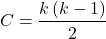
for more on pairwise comparisons, see 10.1 – Compare two independent sample means
For our three group experiment, how many pairwise comparisons can be tested? Therefore,  , and we have
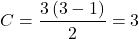
Thus, for our three groups, A, B, and C, there are three possible pairwise comparisons.
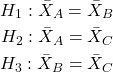
How many pairwise comparisons for a four group experiment? Check your work, you should get  .
The multiple comparison problem
Let’s say that we’re stubborn. We could do many single two-sample t-tests — certainly, your statistical software won’t stop you — this is a situation that calls for statistical reasoning. Here’s why we should not: we will increase the probability of rejecting a null hypothesis when the null hypothesis is true (eg, discussion in Jafari and Ansari-Pour 2019). That is, the chance we will commit a Type I error increases if we do not account for the lack of independence in these sets of pairwise tests evaluated by t-tests. This is multiplicity or the multiple comparison problem.
Review: when we perform a two-sample t-test we are willing to reject a true null hypothesis 5% of the time. This is what is meant by setting the critical probability value (alpha) = 0.05. By “willing” we mean that we know that our conclusions could be wrong because we ar3 working with samples, not the entire population. (Of course at the time, we have no way of actually knowing WHEN we are wrong, but we do want to know how likely we could be wrong!) However, if we compare three population means we have three separate null hypotheses.
HO: one or more of the means are different.
But if we conduct these as separate independent sample t-tests, then we are implicitly making the following null hypothesis statements:
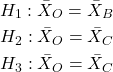
Thus, we have a 5% chance of being wrong for the first hypothesis and/or a 5% chance of being wrong for the second hypothesis and/or a 5% chance of being wrong for the third hypotheses. The chance that we will be wrong for at least one of these hypotheses must now be greater than 5%.
For three separate hypotheses there is a 14% chance of being wrong when we have the probability value for each individual t-test set at α = 0.05. How did we get this result? The point is that these tests are not independent, they are done on the same data set, therefore you can’t simply apply the multiplication probability rule.
Here’s how to figure this: for the set of three hypotheses, the probability of incorrectly rejecting at least one of the null hypotheses is

So, for three t-tests on the same experiment, the Type I error overall tests (experiment-wise) is actually 14% not 5%. It gets worse as the number of combinations (groups and therefore hypotheses) increases. For four groups, Type I error is actually

That’s 26.5%, not 5%.
If we have just five populations means to compare the probability of rejecting a null hypothesis when it is true climbs to 60%! How did this happen? The probability or correctly rejecting all of them is now

So, the probability of incorrectly rejecting one test (Type I error) is now

instead of the 5% we think we are testing.
The key argument for why you must use ANOVA to analyze multiple samples instead of a combination of t-tests!! ANOVA guarantees that the overall error rate is the specified 5%.
Why is the Type I error not 5% for each test? Because we conducted ONE experiment, we can conduct only ONE test (we could be right, we could be wrong 5% of the time). If we conduct the experiment over again, on new subjects, each time resulting in new and therefore independent data sets, then Type I error = 5% for each of these independent experiments.
Now, I hope I have introduced you to the issue of Type I error at the level of a single comparison and the idea of an experiment, holding Type I error-rates at 5% across all hypotheses to be evaluated in an experiment. You may wonder why anyone would make this mistake now. Actually, people make this “mistake” all the time and in some fields like evaluating gene expression for microarray data, this error was the norm, not the exception (see for example discussion of this in Jeanmougin et al 2010).
To conclude, if one does multiple tests on the same experiment, whether it is t-tests or some other test for that matter, then our subsequent tests are related. This is what we mean by independence in statistics — and there are many ways that nonindependence may occur in experimental research. For example, we introduced the concept of pseudoreplication, when observations are treated as if they are independent, but they are not (see Chapter 5.2). The “multiple comparison problem” specifically refers to the lack of independence when all the data set from a single experiment is parsed into lots of separate tests. Philosophically, there must be a logical penalty — and that is reflected in the increase in Type I error.
Clearly something must be done about this!
Corrections to account for the multiple comparisons problem
The family-wise (aka experiment-wise) error rate for multiple comparisons is kept at 5%, and each individual-wise comparison is compared against a more strict (ie, smaller Type I error rate). Put another way, the family-wise error rate is the chance of a number of false positives: making a mistake when we consider many tests simultaneously. The simplest correction for the individual-wise error rate is the Bonferroni correction: test each individual comparison at Type I error equal to  , where C is the number of comparisons. The Šidák correction,
 , and the Holm-Bonferroni method are alternatives with reportedly better statistical properties (eg, reduced Type II error rates; Ludbrook 1998, Sauder and DeMars 2019).
ANOVA is a solution
One possible solution for getting the correct experiment-wise error rate: adjust for differences in probability for multiple comparisons with the t-test. We used post-hoc tests presented above: you could evaluate the tests after accounting for the change in Type I error. This is what is done in many cases. For example, in genomics. In the early days of gene expression profiling by microarray, it was common to see researchers conduct t-tests for each gene. Since microarrays can have thousands of genes represented on the chip, then these researchers were conducting thousands of t-tests, arranging the t-tests by P-value and counting the number of P-values less than 5% and declaring that the differences were statistically significant.
This error didn’t stand long, and there are now many options available to researchers to handle the “multiple comparisons” problem (some probably better than others, research on this very much an ongoing endeavor in biostatistics). The Bonferroni correction was an available solution, largely replaced by the Holm (aka Holm-Bonferroni) method (Holm 1979). Recall that the Bonferroni correction judged individual p-values statistically significant only if they were less than , where, again, α is the family-wise error rate (eg, α = 5%) and C was the number of comparisons. The Holm method orders the C p-values from lowest to highest rank. The method then evaluates lowest p-value, if less than , then reject hypothesis for that comparison. Proceed to next p-value, if less than , then reject hypothesis for that comparison, and so on until no more comparisons are less than .
A MUCH better alternative is to perform a single analysis that takes the multiple-comparisons problem into account: Single Factor ANOVA, also called the one-way ANOVA, plus the post-hoc tests with error correction. We introduce one-way ANOVA in the next section. Post-hoc tests are discussed in Chapter 12.6.
Questions
- You should be able to define and distinguish how Bonferoni correction, Dunnett’s test, and Tukey’s test methods protect against inflation of Type I error.
- What will be the experiment-wise error rate for an experiment in which there are only two treatment groups?
- Experiment-wise error rate may also be called _______________ error rate.
- List and compare the three described posthoc approaches to correct for multiple comparison problem,
- Glycophosphate-tolerant soybean is the number one GMO (genetically modified organism) crop plant worldwide. Glycophosphate is the chief active ingredient in Roundup, the most widely used herbicide. A recent paper examined “food quality” of the nutrient and elemental composition of plants drawn from fields which grow soy by organic methods (no herbicides or pesticides) and GMO plants subject to herbicides and pesticides. A total of 28 individual t-tests were used to compare the treatment groups for different levels of nutrients and elements (eg, vitamins, amino acids, etc.,); the authors concluded that 10 of these t-tests were statistically significant at Type I error rate of 5%. Discuss the approach to statistical inference by the authors of this report; include correct use of the terms experiment-wise and individual-wise in your response and suggest an alternative testing approach if it is appropriate in your view.
- In Chapter 4.2 we introduced a data set from an experiment. The experiment looked at DNA damage quantified by measuring qualities in a Comet Assay including the Tail length, the percent of DNA in the tail, and olive moment. The data set is copied to end of this page. In the next chapter I’ll ask you to conduct the ANOVA on this experiment. For now, answer the following questions.
a. What is the response variable? Defend your choice(s).
b. Why is this an ANOVA problem? Include as part of your explanation a statement of the null hypothesis.
Quiz Chapter 12.1
The need for ANOVA
Data used in this page
comet assay dataset
| Treatment | Tail | TailPercent | OliveMoment* |
|---|---|---|---|
| Copper-Hazel | 10 | 9.7732 | 2.1501 |
| Copper-Hazel | 6 | 4.8381 | 0.9676 |
| Copper-Hazel | 6 | 3.981 | 0.836 |
| Copper-Hazel | 16 | 12.0911 | 2.9019 |
| Copper-Hazel | 20 | 15.3543 | 3.9921 |
| Copper-Hazel | 33 | 33.5207 | 10.7266 |
| Copper-Hazel | 13 | 13.0936 | 2.8806 |
| Copper-Hazel | 17 | 26.8697 | 4.5679 |
| Copper-Hazel | 30 | 53.8844 | 10.238 |
| Copper-Hazel | 19 | 14.983 | 3.7458 |
| Copper | 11 | 10.5293 | 2.1059 |
| Copper | 13 | 12.5298 | 2.506 |
| Copper | 27 | 38.7357 | 6.9724 |
| Copper | 10 | 10.0238 | 1.9045 |
| Copper | 12 | 12.8428 | 2.5686 |
| Copper | 22 | 32.9746 | 5.2759 |
| Copper | 14 | 13.7666 | 2.6157 |
| Copper | 15 | 18.2663 | 3.8359 |
| Copper | 7 | 10.2393 | 1.9455 |
| Copper | 29 | 22.6612 | 7.9314 |
| Hazel | 8 | 5.6897 | 1.3086 |
| Hazel | 15 | 23.3931 | 2.8072 |
| Hazel | 5 | 2.7021 | 0.5674 |
| Hazel | 16 | 22.519 | 3.1527 |
| Hazel | 3 | 1.9354 | 0.271 |
| Hazel | 10 | 5.6947 | 1.3098 |
| Hazel | 2 | 1.4199 | 0.2272 |
| Hazel | 20 | 29.9353 | 4.4903 |
| Hazel | 6 | 3.357 | 0.6714 |
| Hazel | 3 | 1.2528 | 0.2506 |
Tail refers to length of the comet tail, TailPercent is percent DNA damage in tail, and OliveMoment refers to Olive's (1990), defined as the fraction of DNA in the tail multiplied by tail length
Chapter 12 contents
11.3 – Factors influencing statistical power
Introduction
Components of an experimental design that may influence statistical power include:
- α (probability of committing a Type I error).
As the probability of a Type I error increases, the probability of a Type II error decreases. Therefore, as α gets bigger, power gets decreases. - σ, the variance in the population
Statistical power decreases as variability increases. - Effect size
The effect size is a measure of the differences between two or more groups considered biologically important; its difficult to have lots of power to detect very small differences. - Sample size
As n increases, power increases
Size of alpha (Type I error)
When we introduced the idea of Type I error, alpha, it followed a story about Challenger, the space shuttle that disintegrated after failure of O-rings allowed hot gasses to cross joints in the rockets. If we adopt a Type I error rate of 5% in our rocket designs, then failure is expected at one in twenty launches. That rate clearly is unacceptable, so the logical extension of this thinking would be to decrease the Type I error rate. Unfortunately, this comes at the expense of increasing our risk of Type II error. Thus, decreasing Type I error decreases statistical power.
Variance
If the range of values for individuals in the samples are great, then it should not be surprising that the power to distinguish between sample means from the groups will be low. Conversely, if the variance for a sample is small, then the precision of the estimated sample mean will increase, and, therefore, the power will increase.
Effect size
Effect size deserves some more comments. If we are thinking cause/effect, then we are asking whether or not our independent variable explains a lot of variation in the response (dependent) variable. If there is a strong link between the independent and dependent variable, then the effect size will be large and small numbers of observations will be needed.
There are various ways to estimate effect size, but the simplest is a variation of the t-test (Cohen’s d).

The formula would be different for ANOVA (involves the mean squares), but you get the idea. By convention, an effect size of about 0.2 would be “small,” 0.5 would be “medium,” and an effect size greater than 0.8 would be “large.”
Sample size
This is the area of course where the experimenter has control. We can choose how many individuals are assigned to treatment groups. The Central Limit Theorem basically states that you can use the normal distribution to predict how likely an individual observation is in relation to a sample mean even if the sample distribution is not normally distributed. The larger the number of individuals in the sample from a population, the more confidence we have about making this assumption. Translation: sample size directly impacts standard error of the calculated statistic. Recall our equation for the standard error of the mean.
Alternatives to Cohen’s d
Glass’s g
Hedges’ gu
Keselman and colleagues’ dj
estimators based on trimmed mean and Winsorized variances.
Questions
- The Central limit Theorem can be invoked when we have large samples of observations. In this subchapter we state that increase sample size increases statistical power. Discuss and contrast these two characteristics of large sample size on statistical inference.
- How many samples are enough? Some statistical textbooks will cite a rule of 30. With respect to factors that affect statistical power, discuss the limitations of adopting such a rule to design an experiment.
Quiz Chapter 11.3
Factors influencing statistical power
Chapter 11 contents
- Introduction
- What is Statistical Power?
- Prospective and retrospective power
- Factors influencing statistical power
- Two sample effect size
- Power analysis in R
- References and suggested readings
10.3 – Paired t-test
Introduction
Good experiments include controls. Interested in a new treatment for weight loss? Define a control group to compare the weight loss by a group using the new product. In many cases, the best control is the individual.
Consider now a basic experimental design, the randomized crossover trial (Fig 1), introduced in Chapter 2.4.

Figure 1. A two group Randomized Crossover Trial.
Subjects randomly selected from population of interest, then again once recruited into one of two treatment arms: arm 1, subjects first receive the experimental treatment, then some time later the subjects receive the control treatment; arm 2, subjects first receive the control treatment, then some time later the subjects receive the experimental treatment. Note the difference between this paired or repeated measures design and the independent sample design (see Chapter 10.1). Repeated measures designs have many advantages; we discuss them further in Chapter 14.6. At the start, repeated measures designs have greater statistical power compared to cross-sectional (independent) sample designs.
Many experiments are designed so that subjects receive all treatments and responses are gauged against the initial values recorded on the subjects. Repeated measures statistical tests, like the paired t-test, are needed however to analyze the data. These types of statistical procedures are similar to the two sample independent t-test that we discussed earlier.
However, there is an important difference between these two types of statistical procedures. For the two independent sample t-test the samples are unpaired: we observed one variable on some individuals assigned to two different groups. These groups might be
- Two locations where we measure plants or animals
- A treatment (or experimental) group with a control group.
- Expression of cytokeratin genes (eg, ΔΔCT, fold-change) from breast cancer patients compared to healthy donor subjects (Andergassen et al 2016).
The point is that samples in one group are not the same samples in the second group.
In the paired t-test we have two groups but the observations in these two groups are paired. Paired means that there is some relationship between one observation in the first sample and one observation in the second sample (every observation in one sample must be paired with one observation in another sample).
For example, weight change in humans before and after a change in diet could be performed as a paired analysis. Each subject’s weight before the diet was “paired” with the same subject’s weight after the diet.
Another example comes from genetics. Siblings or Monozygotic twins or clones, strains or varieties of plants or animals can be Paired in an experiment.
- You can give one of the twins a particular diet, or the plant or animal clones or strains can be raised in a particular environment (nutrient)
- The other twin or plant or animal clone or variety can serve as a type of control by providing a normal diet or normal environment.
Another example is a study of environmental pollution on cancer rates in many different communities.
- The researchers selects pairs of communities with similar characteristics for many socioeconomic factors.
- Each pair of communities differed with respect to the proximity to a known source of pollution: one of the pair was close to a source of pollution and one of the pair was far from a source of pollution.
The purpose of pairing in this example is to attempt to “control” for all the socioeconomic factors that might contribute to cancer but they did not want to directly measure. These other factors should be similar for each member of the pair.
Example: How repeatable is human running performance?
The subheading is misleading — we leave “repeatability” or, do individuals perform consistently to another time (see Chapter 12.3 – Fixed effects, random effects, and agreement). Here, we focus on a different question — we test whether mean performance differs across repeated trials. This may seem a subtle difference, but consistency asks the question if performance, whether it is answering questions on an exam or running times for a race, is stable across trials. Testing the means of first and second trials asks a different question: we test for a trend in performance, which may reflect learning.
Here’s an example in which a measure was taken twice for the same individuals. The data are running speed or pace during 5K race held annually on Oahu for a selected sample of female runners with repeat race times (20 – 29 years old). The race was run annually on Oahu, and the data reported are the pace for the first race and the second race, which occurred a year later (Jamba Juice – Banana Man Chase, Ala Moana Beach Park, data extracted from source, https://timelinehawaii.com).
Table 1. 5K pace times (kph) for 15 women (20 – 29 years)
| ID | First race | Second race |
|---|---|---|
| 1 | 15.28 | 15.61 |
| 2 | 11.22 | 11.19 |
| 3 | 8.80 | 9.14 |
| 4 | 8.88 | 5.46 |
| 5 | 9.81 | 10.50 |
| 6 | 6.12 | 5.69 |
| 7 | 8.31 | 8.71 |
| 8 | 6.26 | 7.42 |
| 9 | 17.16 | 16.41 |
| 10 | 16.23 | 15.82 |
| 11 | 5.90 | 7.12 |
| 12 | 8.31 | 10.48 |
| 13 | 5.93 | 8.64 |
| 14 | 10.54 | 5.99 |
| 15 | 9.53 | 8.69 |
Note 1: We’ll return to this data set in Chapter 15.3
Load the data into R as an unstacked data set. Data available at end of this page or click here.
Begin with description and exploration of the data. Start with histograms to get a sense of the sample distributions (hint: we’re looking to see if the data looks like it could come from a normal distribution, see Chapter 13.3 Assumptions) (Fig 2).
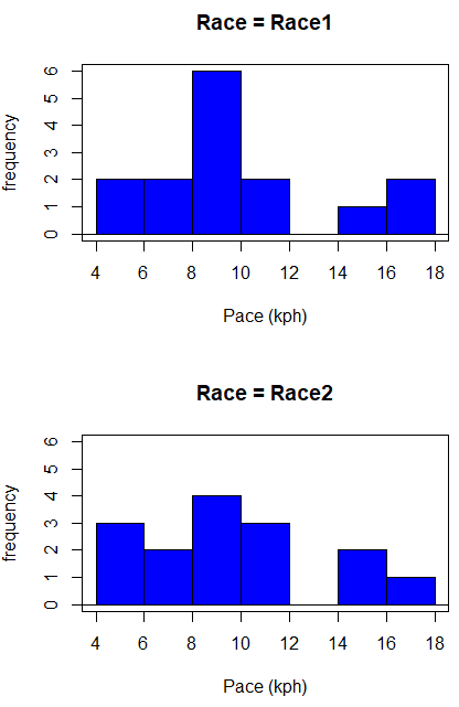
Figure 2. Histograms shows the distribution of 5K running times of 15 women who ran the race twice.
R code (stacked data set, then used defaults R Commander to make the histogram, then modified the code and submitted modified code to make Fig 1)
with(stackExCh10.3, Hist(obs, groups=Race, scale="frequency", breaks="Sturges", col="blue",
xlab="Time (min)", ylab="Frequency")))
Conclusion? The histograms don’t look normally distributed so we keep this in mind as we proceed. (See Chapter 13 – Assumptions of parametric tests for additional information about assumptions.)
A box plot comparing the first and second pace times (Fig 3).
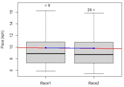
Figure 3. Box plot of race speed (kph) for 15 women 5K in two successive years.
I added a trend line (linear regression, see Chapter 17, red line) and connected the averages (blue line) for visual emphasis — no differences between the means — but note that one wouldn’t do this as part of an analysis (see Chapter 4 discussion).
R code for Fig 2
Boxplot(obs~Race, data=stackExCh10.3, id=list(method="y"), xlab="", ylab="Pace (kph)") #boxplot was made in Rcmdr
abline(lm(obs ~ as.numeric(Race), data=stackExCh10.3), col="red", lwd=2)
means <- tapply(obs, Race, mean)
points(1:2, means, pch=7, col="blue")
lines(1:2, means, col="blue", lwd=2)
The box plot works to show the median difference, but loses the paired information. A nice package called PairedData has several functions that work well with paired data, for example a profile plot (Fig 4). A profile plot is useful for showing an association between paired data.
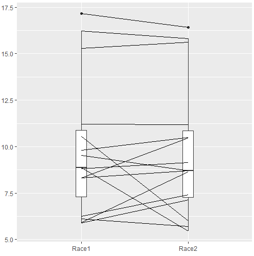
Figure 4. Profile plot, PairedData package.
R commands for Figure 4.
require(PairedData)
attach(example.ch10.3) # remember to attach dataframe so you don't have to call variables like example.ch10.3$Race1
races <- paired(Race1, Race2)
plot(races, type = "profile")
Paired t-test calculation
The paired t-test is a straight-forward extension of the independent sample t-test; the key concept is that the two samples are no longer independent, they are paired. Thus, instead of mean of group 1 minus mean of group two, we test the differences between sample 1 and sample 2 for each paired observation.

- Compute the differences between the Paired Samples (as in tables above)
- Calculate the MEAN difference score,
 : in the previous example = -0.094 kmh
- Calculate the degrees of freedom df = # pairs – 1 = n – 1, where n is the number of pairs
- Calculate the standard error of the mean of d.

where

- Calculate the test statistic for paired data

- Compare to the Critical Value in Table C. 4 (Appendix Table 2)
- Find the Critical Value = t α (2), df
Try as difference instead of paired
Before you answer, take a look at the box plot of the mean difference between the repeat measures of 5K pace for the 15 women (Fig 5).
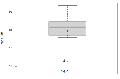
Figure 5. Box plot of differences, Red dotted lines shows the null hypothesis.
Note 2: Figure 5 is appropriate for diagnostics, but not for publication, per our discussions in Chapter 4.
Create a new variable, raceDiff, equal to Race2 minus Race1. Then, use the one sample T-test on raceDiff. I’ll leave you to complete the work (Question 2).
R code
t.test(Race1, Race2, paired = TRUE, alternative = "two.sided")
R output
Paired t-test

data: Race.1 and Race.2
t = 0.19389, df = 14, p-value = 0.849
alternative hypothesis: true difference in means is not equal to 0
95 percent confidence interval:
-0.9491017 1.1377521
sample estimates:
mean of the differences
0.09432517
Rcmdr, paired t-test
Rcmdr: Statistics → Means → Paired t-test…
Note: your two groups must be in two different columns (unstacked!) to run this version of the test.
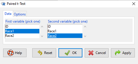
Figure 6. R Commander Paired t-test menu, Rcmdr version 2.7.
After selecting the variables, set null hypothesis after clicking on Options tab (Fig 6).
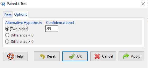
Figure 7. R Commander Paired t-Test options, select null hypothesis.
Click OK to proceed. Results will be the same as the output listed above.
the following text needs to be updated
Interpret the results.
So, what can we conclude about the null hypothesis? Interpret the 95% CI, the T-test statistic, and the P-value.
Do not ignore sample dependence
What if we ignored the repeated measures design and treated the first and second races as independent? The important concept here is to ask, what would have happened if we had done a two independent sample t-test instead?
Let’s run the analysis again, this time incorrectly using the independent sample t-test. We need to manipulate the data set before we do.
Manage your data: Stack the data
This is a good time to share how to Stack data in R. If you look at our active data set, the results of the two trials are in two different columns. In order to run the independent sample t-test we need the data in one column (with a label column).
stackExCh10.3 <- stack(example.ch10.3[, c("Race1","Race2")])
names(stackExCh10.3) <- c("obs", "Race")
Rcmdr: Data → Active data set → Stack variables in data set…
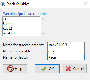
Figure 8. R Commander: Stack worksheet. Select the two variables, Race1 and Race2.
I entered values for name of the new data set, the new variable, and the name for the factor (label) column.
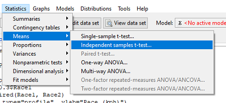
Figure 9. R Commander, select independent sample t-Test …
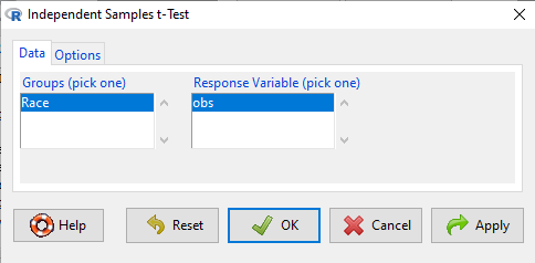
Figure 10. R commander, independent sample t test menu.
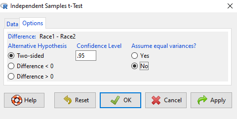
Figure 11. R Commander, select options for independent sample t-Test (assume equal variance).
Here are the results of the independent sample t-test from R.
t.test(obs~Race, alternative='two.sided', conf.level=.95, var.equal=TRUE, + data=stackCh10.3)

Two Sample t-test
data: obs by Race
t = 0.070645, df = 28, p-value = 0.9442
alternative hypothesis: true difference in means is not equal to 0
95 percent confidence interval:
 -2.640719 2.829369
sample estimates:
mean in group Race1 mean in group Race2
 9.886342 9.792017
End R output
In this case, we would have reached the same general conclusion, but the p-values are different. The p-value from the paired t-test was about 0.85 whereas the p-value from the independent sample t-test was higher, nearly 0.95, suggesting little difference between the two trials.
While the general conclusion holds, this time, that there were no statistically significant difference between the means for first and second trials. However, it won’t always work out that way. And besides, if you treated the paired data as independent, you’ve clearly violated one of the assumptions of the test.
Take a look at the degrees of freedom for the two analyses. By ignoring the pairing of samples we gain twice the number of degrees of freedom … that can’t both be right. The way to distinguish between the two is to go back to the experimental units.
Question: What are the sampling units in the case of repeat measures on individuals: the individuals themselves? the pairs of burst speed trials? something else?
it is important to note that the paired t-test is still the best for this situation because it accurately reflects the experiment — individuals were measured twice, therefore the two groups (trial 1 and trial 2) are not independent! Thus, the p-value from the paired t-test correctly reflect our best analyses of the test of the null hypothesis because the correct degrees of freedom were 14 and not 28.
In the case of the independent sample t-test we necessarily make the assumption that the two groups are independent — that is, that they are measured on different sampling units (eg, different individuals or subjects). In statistical terms, that means that you assume that the correlation between trial results is equal to zero. By incorrectly choosing an independent sample test in these repeated measures cases, I would make two null hypotheses: (1) that the means are the same and (2) that the correlation between repeat measures is zero. The problem? The t-test only evaluates the first hypothesis (means).
Questions
- Refer to Figure 6 again and related data set. Were runners faster the second year or the first year running the 5k? What about the points labeled 4 and 14? What was the average difference between first and second races?
- Complete the test of the null hypothesis of no difference between race 1 and race 2 (
raceDiff) with the one sample t-test. Set up a table to compare the test statistic, df, and p-values for results from paired t test, one sample t-test, and independent sample t-test. How do these results compare? - I’ve called the observed value “pace,” but runners would know that pace is actually amount of time per kilometer, not the total time over 5k, which is what I called pace.
- Create a new variable and report average pace for Race1 and Race2.
- Redo the paired analysis, including box plot, on your new variable.
- What is the null hypothesis for your new variable?
- Summarize your results and add to the table you created for question 2.
- Redo the two plots in Figure 2 so that the two histograms are on the sample plot. Instructions and examples were provided in Chapter 4.2.
Quiz Chapter 10.3
Paired t-test
Data set
example.ch10.3 <- read.table(header=TRUE, text = "
ID Race1 Race2
1 15.28 15.61
2 11.22 11.19
3 8.80 9.14
4 8.88 5.46
5 9.81 10.50
6 6.12 5.69
7 8.31 8.71
8 6.26 7.42
9 17.16 16.41
10 16.23 15.82
11 5.90 7.12
12 8.31 10.48
13 5.93 8.64
14 10.54 5.99
15 9.53 8.69
")
Chapter 10 contents
10.2 – Digging deeper into t-test Plus the Welch test
Introduction
We need to spend some more time with the independent sample t-test; by tearing it apart, we can learn about how parametric tests work in general.
Our assumptions for the independent sample t-test are like the one-sample t-test the data must be continuous and normally distributed (one of our standard assumptions for parametric tests, see Chapter 13). The formula is very similar to the one-sample t-test, except that now we have two sample means and the formula for the standard error (SE) has also changed.

We see that the test statistic t is large if the numerator is large compared to the denominator. Large values of t will be evidence in favor of rejecting the null hypothesis.
The numerator is straightforward: we subtract one sample mean from the other — if there is no difference between the samples, then this difference will be close to zero.
The denominator requires additional discussion. What is it called? It is the pooled standard error of the mean (pooled SEM). Provided the assumption of equal variances holds — an additional standard assumptions for parametric tests, see Chapter 13 — then sample variances estimate the population variance and we can use this information to our advantage to best test the hypothesis about the sample means. In other words, we don’t have to lose a degree of freedom to account for differences in variability for the two groups (see Welch test). More degrees of freedom means more statistical power to test the null hypothesis and at the same time, more confidence that the test is performing to its best.
Lets break down the pooled standard error of the mean in order to see how the assumption of equal variances affects the t-test. We assume that 
Recall that

Now we want a “pooled SE” that is the pooled standard error for both samples. The variance of the difference between the means can be written as
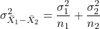
First we need to calculate the pooled variance. where v1 and v2 are degrees of freedom for sample one and sample two, respectively.
Note 1This is just simply a combined formula of the sample variance.
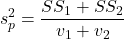
What is SS? The sum of squares , where SS1 and SS2 refer to sum of squares for each of the two groups.
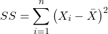
You should recognize SS from your definition of the sample variance, Chapter 3.3.
And the standard error for the difference between two means can now be written as So the 2-sample t-test can be written to reflect the pooled sample standard error of the difference between two sample means. We can see how unequal sample size is accommodated by the t-test.
Conducting the test by hand follows the same form as the one-sample t-test. Find the degrees of freedom (DF), but now for each sample.
Finally we evaluate with the critical value in Table (Appendix, Table of Student’s t distribution) and compare the t test statistic against the critical value with the appropriate degrees of freedom.
Because this is the t-test, again, we are assuming that the variances are the same between the two populations (homoscedasticity) and this allows us to pool the variance. As it turns out, the T-test is not overly sensitive to other deviations from the assumptions, but if the variances are in fact different, then the standard formula may yield incorrect Type I error rates compared to stated probability level (α).
However, it would be poor statistical choice to use a test where there are alternatives. This is why in part that R (Rcmdr) sets as the default for the t-test that variances are unequal! In fact, R does not do a t-test unless you change the default to assume equal variances, which, as we now know, is the t-test.
Welch test
What to do when assumptions to t-test are not met? Many options have been proposed, and Welch’s approximate t is a good alternative to the two-sample t-test — it would be appropriate if the normal assumption still held.
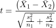
The degrees of freedom for the Welch’s test are now
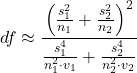
Note 2: The Welch test removes the pooled estimate of the standard error, replaces with both variance estimates directly.
As a default option, R and Rcmdr uses a variation of Welch’s test when you select to do the t-test without making the assumption of equal variance (Fig 1).
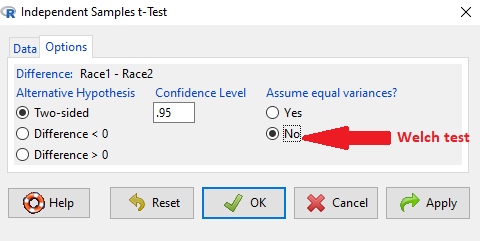
Figure 1. Screenshot Rcmdr t-test options. Default is “No” for Assume equal variances, ie, the Welch test.
The Welch test is not a nonparametric test, it is a different formulation of the t-test.
Justification for beginning with t-test
It’s unlikely that you will need the t-test in today’s research climate. Data sets are large, experiments are complex with multiple variables and samples. Why do we have to consider the t-test, and then a separate test in the case for unequal sample size? I view it as a teaching moment. It makes the general point that ALL statistical tests make assumptions about how the calculations are done and as to the nature of the data set.
This is our first experience with what to do if there is a violation of an assumption of parametric tests (see Chapter 13). Here, the assumption is that the two groups have equal sample size. When they do not, the standard t-test tends to biased estimates. On the other hand, if the assumptions are met, the standard test is the best test because it has more power to do what we intended — that is, it is best at the actual test of the null hypothesis! Take heart — this point is not always appreciated even by scientists (cf. Fagerland 2012).
Note 3: Expert advice will differ here, but you can always calculate the test statistic, even if the assumptions do not hold. The problem, the concern is with the interpretation.
Let’s us approach the problem of violation of assumptions in a couple of ways as an introduction to how, in general, to approach choice of statistical tests.
- Power of a test. Much current statistical research focuses on learning about how a particular statistical test works when assumptions are violated. Thus, in addition to learning what tests are designed to do, we need to consider the effects of violations of assumptions on the performance of the test (namely, is the Type I error at the stated alpha level?). This is a matter of statistical power; power of a test reflects how able the test is to get you the correct result even if assumptions are violated. Often tests perform well if sample sizes are large despite violation of assumptions. We mention without proving that the 2-sample T-test is robust to violations of normality assumption, to requirement for equal sample size, and even to unequal variances. But good experimental design attempts to meet the assumptions because the test does better!
- Alternate forms of some tests are available to handle some aspects of test violations. For example, the simple 2-sample T-test can be modified to accommodate different variances (Welch’s formula). Or you must find a different test (eg, nonparametric tests).
In conclusion, all tests begin with consideration of the assumptions. In some cases we can test our assumptions. For example, we learned about testing the assumption of normal distributions of sample data. We can also test the assumption of equal variances.
Questions
- Consider a clinical trial in which resting blood pressure is recorded on hypertensive subjects at the start of the trial, then 6 weeks after subjects have received daily supplements of flaxseed. Thus, for each subject there are two measures of blood pressure, BEFORE and AFTER.
- Write the null hypothesis
- Write the alternative hypothesis
- Justify why or why not the hypothesis should be two tailed. Explain why or why not an independent sample t-test may be used to compare groups.
Quiz Chapter 10.2
Digging deeper into t-test Plus the Welch test
Chapter 10 contents
- Introduction
- Compare two independent sample means
- Digging deeper into t-test Plus the Welch test
- Paired t-test
- References and suggested reading
10.1 – Compare two independent sample means
Introduction
We introduced the concept of comparing a sample statistic (mean) against a population parameter (Chapter 6.7, Normal deviate) or one-sample t-test against a specified mean (eg, from published data or from theory, Chapter 8.5).
Consider now a basic experimental design, the randomized control trial, or RCT (Fig 1), introduced in Chapter 2.4.
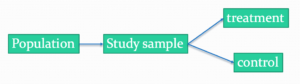
Figure 1. A two group Randomized Control Trial.
Subjects randomly selected from population of interest, then again — random assignment — once recruited into one of two treatment groups. Importantly, subjects belong to one treatment arm only: no subject simultaneously receives the treatment and the control. This is in contrast to the paired design, in which subjects receive both treatments (see Chapter 10.3).
In inferential statistics about an experiment, we are more likely trying to test if sample means are different. For example
- two species grown in common garden, do they differ in growth rate?
- human subjects given a new treatment have better outcomes compare to those receiving a control treatment (eg, placebo).
The equivalent null hypothesis is that two samples are pulled from the same population. We write the null hypothesis as

and the corresponding alternative hypothesis, HA, then must be

Question: Is this a one tailed or two-tailed hypothesis?
Answer: Two-tailed (review Chapter 8.4)
Note 1: In this day and age, there’s really no compelling reason to learn the t-test. First, it is just a special case of the one-way ANOVA, therefore, it’s a special case of the general linear model. Struggling to learn R commands? Well, one solution would be just to learn the general linear model approach — the R function lm() (OK — don’t get too excited — lm() has many options and details). Second, few experiments or observational studies are likely to have only two groups; thus, the temptation to carry out a series of t-tests, taking all groups two at a time, or “pairwise,” while tempting, actually violates a whole bunch of basic statistical rules (discussed in Chapter 12.1). It will also make statisticians go crazy when they see it. That said, if your experiment has but two groups, then by all means, the t-test is a choice. The t-test is also a statistical test that you have likely already used before so we present the discussion here to build on what you may already have learned. We also present the independent t-test as a vehicle.
Worked example
We introduce the two-sample t-test, or better, the independent sample t-test.

where the numerator is the difference between the two sample means and the denominator is the standard error of the differences between the two groups standard errors. The formula for
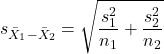
The choice of independent sample over two-sample is best because it emphasizes that the two groups (the two samples), must be comprise of independent sampling units. This is a pretty straight-forward requirement; you have randomly assigned twenty individuals to two groups, a control group (n = 10) and a treatment group (n = 10). Individuals are either in the control group or they are in the treatment group — they cannot simultaneously appear in both groups.
We will work our way through this test by example. For starters, let’s use the same lizard dataset (see Example data set, below), four body mass recordings (grams) each for house geckos (Hemidactylus frenatus, Fig 2) and the Carolina anole (Anolis carolensis, Fig 3), two of many lizard species introduced to Hawaiʻi.

Figure 2. Male Hemidactylus frenatus, central Oahu, M. Dohm.

Figure 3. Male Anolis carolinensis, ʻAkaka Falls, Big Island of Hawaiʻi, M. Dohm.
Example data set
Geckos: 3.186, 2.427, 4.031, 1.995

Anoles: 5.515, 5.659, 6.739, 3.184
Question: How would you go about creating a data frame with the values in long form (stacked worksheet), including a label variable and the body mass?
Note 2: The independent sample t-test in Rcmdr requires a stacked worksheet and not in unstacked worksheet two columns implied by the above pseudo-code. If you need help with worksheet format, then see Part07 in Mike’s Workbook for Biostatistics.
Answer: At the R prompt, type
Geckos <- c(3.186, 2.427, 4.031, 1.995); Anoles = c(5.515, 5.659, 6.739, 3.184) #create two vectors
bmass <- c(Geckos, Anoles)    #combine the two vectors into a single vector holding all of the body mass records
species <- c("gecko", "gecko", "gecko", "gecko", "anole", "anole", "anole", "anole")   #create your label variable
lizards <- data.frame(species, bmass)  #create your data frame
lizards   #print your data frame  species bmass
1   gecko 3.186
2   gecko 2.427
3   gecko 4.031
4   gecko 1.995
5   anole 5.515
6   anole 5.659
7   anole 6.739
8   anole 3.184
Note also that you can enter data into the Data editor by creating the data frame first then adding values. To edit the data frame “lizards” type fix(lizards) at the R prompt, then close the data frame when you have added or changed values as needed.
As always, begin with an exploration of the data, including a graph (Fig 4).
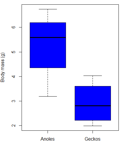
Figure 4. Box plot of lizard body mass.
We can see already that there’s greater spread of data for the Anoles compared to the Geckos, but the median values differ. Small sample sizes can be a problem for analyses as we can only have reduced confidence in our conclusions. However, we press on for the sake of demonstration.
Let’s test the null hypothesis, H0, ie, the two species of lizards have the same mean body mass.
Rcmdr: Statistics → Means → Independent-samples t-test…
In this next image I posted the Rcmdr menu popup for the Independent Samples t-test (Fig 5). Later versions of Rcmdr split the settings for this command into two tabs; the first tab allows for the selection of the variables and setting the hypotheses whereas the second tab, labeled Options, permits additional choices. The default selections need your attention: to actually conduct the t-test you need to answer “No” to the question, “Assume equal variance?” (Fig 6).
Figure 5. Rcmdr menu for Independent sample t-test.
Select the Options tab (Fig 6) to select null hypothesis and to select the t-test and not the Welch-test (which is the default, ie, No to the prompt “Assume equal variances?”).
Figure 6. Rcmdr Options menu for Independent sample t-test.
Let’s look at the results and break down the parts of the test.
t.test(Body.mass~Lizard, alternative='two.sided', conf.level=.95,
+ var.equal=TRUE, data=lizards)

Two Sample t-test

data: Body.mass by Lizard
t = 2.7117, df = 6, p-value = 0.03503
alternative hypothesis: true difference in means is not equal to 0
95 percent confidence interval:
0.2308685 4.4981315
sample estimates:
mean in group Anolis mean in group Gecko
5.27425 2.90975
Consider the R session output above and answer the following questions.
Questions for the worked example
- Which lizard group had the greater mean value, Anolis or Gecko?
- What are the assumptions necessary for you to use the independent sample t-test?
- What does “two-sided” mean?
- What was the null hypothesis?
- Was this a one-tailed or two-tailed test of the null hypothesis?
- What is the value of the test statistic?
- How many degrees of freedom?
- What is the critical value for this test?
- What is the value of the lower limit of the 95% confidence interval?
- What is the value of the lower limit of the 99% confidence interval?
- True or False. If the null hypothesis is accepted, then zero is a value included in the 95% confidence interval.
- Do you accept the null hypothesis? Explain your selection.
Try another example
DNA damage, changes in the chemical structure of nucleotide bases or breakage of the DNA chains, occurs in cells under many circumstances. The comet assay, or single-cell gel electrophoresis, is one method for visualizing and measuring DNA strand breaks in cells. Exposed cells are mixed with a low-melting temperature agarose and placed onto a microscope slide. The cells are then lysed with an alkaline detergent and high salts. When current is applied across the slide, undamaged DNA remains in the nucleus, whereas damaged DNA extends towards the anode to form a comet-like tail, with imaging assisted by including a fluorescent dye like Sybr-Green. Examples of comets are shown below (Fig 7).
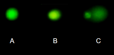
Figure 7. Comet examples. A Intact cell, no DNA damage, B Cell with some DNA damage, a slight tail to the right is evident, C Cell with significant DNA damage, a large tail is evident. M. Dohm.
In an experiment, immortalized lung epithelial cells were exposed to dilute copper solutions for 30 minutes then washed with PBS. The comet assay was applied to these cells and for comparison, to cells without copper exposure but otherwise treated the same way (controls). The data are available at the bottom of this page (scroll down or click here).
Again, you should begin all analyses with an exploration of the data, including a graph (Fig 8).
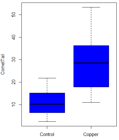
Figure 8. Boxplot of comet tail lengths for cells with and without (control) exposure to copper in the cell medium for 30 minutes.
Let’s look at the R output for the t-test analysis.
    Two Sample t-test

data:  CometTail by Treatment
t = -5.8502, df = 38, p-value = 9.139e-07
alternative hypothesis: true difference in means is not equal to 0
95 percent confidence interval:
 -22.39865 -10.88213
sample estimates:
mean in group Control  mean in group Copper
             11.14533              27.78571
Consider the R session output above and answer the following questions.
Questions for Comet assay data set
- Which cell group had the greater mean value, Copper-exposed or Control-exposed cells?
- What are the assumptions necessary for you to use the independent sample t-test?
- What does “two-sided” mean?
- What was the null hypothesis?
- Was this a one-tailed or two-tailed test of the null hypothesis?
- What is the value of the test statistic?
- How many degrees of freedom?
- What is the critical value for this test?
- What is the value of the lower limit of the 95% confidence interval?
- What is the value of the lower limit of the 99% confidence interval?
- True or False. If the null hypothesis is accepted, then zero is a value included in the 95% confidence interval.
- Do you accept the null hypothesis? Explain your selection.
T test from summary statistics
In some cases you may only have to summary statistics for data, eg, the means and the standard deviations. We can use the equations of the t test to write a simple formula, where the user provides the known means, standard deviations, and sample size. For example, create a simple function with readline for user input.
myTtest <- function() {
   mnx <- as.numeric(readline(prompt="Enter mean of x: "))
   stdevx <- as.numeric(readline(prompt="Enter sd of x: "))
   nx <- as.numeric(readline(prompt="Enter n of x: "))
   mny <- as.numeric(readline(prompt="Enter mean of y: "))
   stdevy <- as.numeric(readline("Enter sd of y: "))
   ny <- as.numeric(readline(prompt="Enter n of y: "))
   myTvalue <- abs(((mnx-mny)-0)/sqrt(((stdevx^2)/nx)+(stdevy^2)/ny))
   myDF <- as.integer(nx+ny-2)
   myPvalue <- pt(myTvalue,myDF,lower.tail=FALSE)*2
   myResults <- c(myTvalue, myDF, myPvalue)
   report <- c("T-test: ", "df: ", "two-tailed p-value: ")
   cat(sprintf("%s %3.3f, ", report, myResults))
}
then run the function by typing myTest() at the R prompt and entering the means, standard deviations, and sample size when prompted.
myTtest()
Enter mean of x: 2.91
Enter sd of x: .895
Enter n of x: 4
Enter mean of y: 5.27
Enter sd of y: 1.497
Enter n of y: 4
T-test: 2.706, df: 6.000, two-tailed p-value: 0.035
P-values from confidence intervals
While we expect certain reporting criteria for published, it is not uncommon that one or more elements are missing. For example, while means plus or minus standard deviations for two groups may be reported, the confidence interval of the difference may not be reported, or, an inexact p-value is reported like “< 0.05,” but we “need” an exact p-value for our meta-analysis. A little math, and these missing statistics can be calculated.
We can use the lizard study as an example; while all of the expected elements were reported, including the p-value (0.03503), let’s say the p value was reported as “statistically significant at p < 0.05.”
We need
lower and upper confidence intervals: 0.2309 and 4.498, respectively.
critical value from t distribution, df = 6 (2 tailed, therefore 0.05/2). A little R code we have:

the standard error, which can be calculated as 
and then the p-value, 
which is pretty close to the result from R (p = 0.03503). The difference is likely due to the small sample size.
Questions
- Don’t forget to work through the Questions for the Comet tail data set (scroll up or click here).
- Microsoft Excel, LibreOffice Calc, and Google sheets spreadsheet software all include t-test functions and return the p-value. Consider two variables big (100, 110, 120, 100, 110, 210, 200) and small (0,1,1,2,0,1,0). (Note — these two groups are obviously very different, calculating a t-test on their difference is silly, just for this question.) If formatting is set to the default two decimal places for Number cell category, the p-value will return as “0.00.” How should you report the p-value in this case?
Quiz Chapter 10.1
Compare two independent sample means
Comet assay data set
| Treatment | CometTail |
| Control | 17.856139 |
| Control | 16.52125 |
| Control | 14.925449 |
| Control | 14.029174 |
| Control | 13.332945 |
| Control | 8.811185 |
| Control | 14.701654 |
| Control | 9.261025 |
| Control | 21.779311 |
| Control | 6.180284 |
| Control | 9.201752 |
| Control | 5.54472 |
| Control | 6.717885 |
| Control | 2.625092 |
| Control | 7.191583 |
| Control | 5.392866 |
| Control | 11.284813 |
| Control | 15.441254 |
| Control | 17.857176 |
| Control | 4.250956 |
| Copper | 53.214287 |
| Copper | 38.92857 |
| Copper | 18.928572 |
| Copper | 30 |
| Copper | 28.928572 |
| Copper | 15.357142 |
| Copper | 17.857143 |
| Copper | 17.5 |
| Copper | 21.071428 |
| Copper | 29.285715 |
| Copper | 28.214285 |
| Copper | 16.785715 |
| Copper | 21.071428 |
| Copper | 37.5 |
| Copper | 38.214287 |
| Copper | 17.857143 |
| Copper | 29.642857 |
| Copper | 11.071428 |
| Copper | 35 |
| Copper | 49.285713 |
Chapter 10 contents
- Introduction
- Compare two independent sample means
- Digging deeper into t-test Plus the Welch test
- Paired t-test
- References and suggested reading
8.6 – Confidence limits for the estimate of population mean
Introduction
In Chapter 3.4 and Chapter 8.3, we introduced the concept of providing a confidence interval for estimates. We gave a calculation for an approximate confidence interval for proportions and for the Number Needed to Treat (Chapter 7.3). Even an approximate confidence interval gives the reader a range of possible values of a population parameter from a sample of observations.
In this chapter we review and expand how to calculate the confidence interval for a sample mean,  . Because is derived from a sample of observations, we use the t-distribution to calculate the confidence interval. Note that if the population was known (population standard deviation), then you would use normal distribution. This was the basis for our recommendation to adjust your very approximate estimate of a confidence interval for an estimate by replacing the “2” with “1.96” when you multiply the standard error of the estimate (SE) in the equation estimate
 . As you can imagine, the approximation works for large sample size, but is less useful as sample size decreases.
Consider ; it is a point estimate of  , the population mean (a parameter). But our estimate of is but one of an infinite number of possible estimates. The confidence interval, however, gives us a way to communicate how reliable our estimate is for the population parameter. A 95% confidence interval, for example, tells the reader that we are willing to say (95% confident) the true value of the parameter is between these two numbers (a lower limit and an upper limit). The point estimate (the sample mean) will of course be included between the two limits.
Instead of 95% confidence, we could calculate intervals for 99%. Since 99% is greater than 95%, we would communicate our certainty of our estimate.
Note 1: Again, the caveats about p-value extend to confidence intervals. See Chapter 8.2.
Question 1: For 99% confidence interval, the lower limit would be smaller than the lower limit for a 95% confidence interval.
- True

- False
When we set the Type I error rate,  (alpha) = 0.05 (5%), that means that 5% of all possible sample means from a population with mean, , will result in t values that are larger than
 OR smaller than
 .
Why the t-distribution?
We use the t-test because, technically, we have a limited sample size and the t-distribution is more accurate than the normal distribution for small samples. Note that as sample size increases, the t-distribution is not distinguishable from the normal distribution and we could use  (Fig 1).
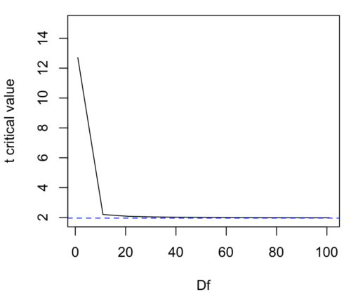
Figure 1. Critical values at Type I rate of 5% of t-distribution  . Blue dashed line is z = 1.96.
Here’s the equation for calculating the confidence interval based on the t-distribution. These set the limits around our estimate of the sample mean. Together, they’re called the 95% confidence interval,  .

Here’s a simplified version of the same thing, but generalized to any Type I level…
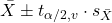
This statistic allows us to say that we are 95% confident that the interval includes the true value for . For this confidence interval you need to identify the critical t value at 5%. Thus, you need to know the degrees of freedom for this problem, which is simply  , the sample size minus one.
It is straightforward to calculate these by hand, but…
Set the Type I error rate, calculate the degrees of freedom (df):
 samples for one sample test
- pairs of samples for paired test
 samples for two independent sample test
and lookup the critical value from the t table (or from the t distribution in R). Of course, it is easier to use R.
In R, for the one tail critical value with seven degrees of freedom, type at the R prompt
qt(c(0.05), df=7, lower.tail=FALSE)
[1] 1.894579
For the two-tail critical value
qt(c(0.025), df=7, lower.tail=FALSE)
[1] 2.364624
Or, if you prefer to use R Commander, then follow the menu prompts to bring up the t quantiles function (Fig 2 and Fig 3).
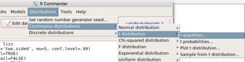
Figure 2. Drop down menu to get t-distribution.
Note 2: Quantiles divide probability distribution into equal parts or intervals. Quartiles have four groups, deciles have ten groups, and percentiles have 100 groups.
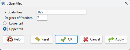
Figure 3. Menu for t quantiles, with values entered for the two-tail example.
You should confirm that what R calculates agrees with the critical values tabulated in the Table of Critical values for the t distribution provided in the Appendix.
A worked example
Let’s revisit our lizard example from last time (see Chapter 8.5). Prior to conducting any inference test, we decide acceptable Type I error rates (cf justify alpha discussion in Ch8.1); For this example, we set Type I error rate to be 1% for a 99% confidence interval.
The Rcmdr output was
t.test(lizz$bm, alternative='two.sided', mu=5, conf.level=.99)
data: lizz$bm
t = -1.5079, df = 7, p-value = 0.1753
alternative hypothesis: true mean is not equal to 5
99 percent confidence interval:
1.984737 6.199263
sample estimates:
mean of x
4.092
Sort through the output and identify what you need to know.
Question 1: What was the sample mean?
- 5
- -1.5079
- 7
- 0.1753
- 1.984737
- 6.199263
- 4.092
Question 2: What was the most likely population mean?
- 5
- Answer
- -1.5079
- 7
- 0.1753
- 1.984737
- 6.199263
- 4.092
Question 3: This was a “one-tailed” test of the null hypothesis?
- True
- False
The output states “alternative hypothesis: true mean is not equal to 5” — so it was a two-tailed test.
Question 4: What was the lower limit of the confidence interval?
- 5
- -1.5079
- 7
- 0.1753
- 1.984737
- 6.199263
- 4.092
The 99% confidence interval,  , is
 , which means we are 99% certain that the population mean is between
 (lower limit) and
 (upper limit). In Chapter 8.5 we calculated the , is
 .
Confidence intervals by nonparametric bootstrap sampling.
Bootstrapping is a general approach to estimation or statistical inference that utilizes random sampling with replacement (Kulesa et al. 2015). In classic frequentist approach, a sample is drawn at random from the population and assumptions about the population distribution are made in order to conduct statistical inference. By resampling with replacement from the sample many times, the bootstrap samples can be viewed as if we drew from the population many times without invoking a theoretical distribution. A clear advantage of the bootstrap is that it allows estimation of confidence intervals without assuming a particular theoretical distribution and thus avoids the burden of repeating the experiment. Which method to prefer? For cases where assumption of a particular distribution is unwarranted (eg, what is the appropriate distribution when we compare medians among samples?), bootstrap may be preferred (and for small data sets, percentile bootstrap may be better). We cover bootstrap sampling of confidence intervals in Chapter 19.2 Bootstrap sampling.
Conclusions
The take home message is simple.
- All estimates should — must? — be accompanied by a Confidence Interval
- The more confident we wish to be, the wider the confidence interval will be
Note that the confidence interval concept combines DESCRIPTION (the population mean is between these limits) and INFERENCE (and we are 95% certain about the values of these limits). It is good statistical practice to include estimates of confidence intervals for any estimate you share with readers. Any statistic that can be estimated should be accompanied by a confidence interval and, as you can imagine, formulas are available to do just this. For example, earlier this semester we calculated NNT.
Questions
- To gain practice with calculations of confidence intervals, calculate the approximate confidence interval, the 95% and the 99% confidence intervals based on the t distribution, for each of the following.
-
- = 13,
 = 1.3,
 = 10
- = 13, = 1.3, = 30
- = 13, = 2.6, = 10
- = 13, = 2.6, = 30
Quiz Chapter 8.6
Confidence limits for the estimate of population mean
Chapter 8 contents
- Introduction
- The null and alternative hypotheses
- The controversy over proper hypothesis testing
- Sampling distribution and hypothesis testing
- Tails of a test
- One sample t-test
- Confidence limits for the estimate of population mean
- References and suggested readings
8.5 – One sample t-test
Introduction.
We’re now talking about the traditional, classical two group comparison involving continuous data types. Thus begins your introduction to parametric statistics. One sample tests involve questions like, how many — what proportion of — people would we expect are shorter or taller than two standard deviations from the mean? This type of question assumes a population and we use properties of the normal distribution and, hence, these are called parametric tests because the assumption is that the data has been sampled from a particular probability distribution.
However, when we start asking questions about a sample statistic (eg, the sample mean), we cannot use the normal distribution directly, ie, we cannot use Z and the normal table as we did before (Chapter 6.7). This is because we do not know the population standard deviation and therefore must use an estimate of the variation (s) to calculate the standard error of the mean.
With the introduction of the t-statistic, we’re now into full inferential statistics-mode. What we do have are estimates of these parameters. The t-test — aka Student’s t-test — was developed for the purpose of testing sample means when the true population parameters are not known.
Note 1: It’s called Student’s t-test after the pseudonym used by William Gosset.
The equation of the one sample t-test. Note the resemblance in form with the Z-score!

where  is the sample standard error of the sample mean (SEM).
For example, weight change of mice given a hormone (leptin) or placebo. The  , but under the null hypothesis, the mean change is “really” zero (
 ). How unlikely is our value of 5 g?
Note 2: Did you catch how I snuck in “placebo” and mice? Do you think the concept of placebo is appropriate for research with mice, or should we simply refer to it as a control treatment? See Ch5.4 – Clinical trials for review.
Speaking of null hypotheses, can you say (or write) the null and alternative hypotheses in this example? How about in symbolic form?
We want to know if our sample mean could have been obtained by chance alone from a population where the true change in weight was zero.
and
and we take these values and plug them into our equation of the t-test
Then recall that Degrees of Freedom are DF = n – 1 so we have DF = 20 – 1 = 19 for the one sample t-test. And the Critical Value is found in the appropriate table of critical values for the t distribution (Fig 1)
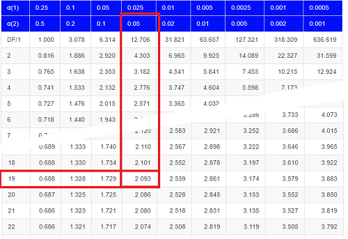
Figure 1. Table of a portion of the Critical values of the t distribution. Red selections highlight critical value for t-test at α = 5% and df = 19.
Note 3: See our table of critical values of t distribution.
Or, and better, use R
qt(c(0.025), df=19, lower.tail=FALSE)
where qt() is function call to find t-score of the pth percentile (cf 3.3 – Measures of dispersion) of the Student t distribution. For a two tailed test, we recall that 0.025 is lower tail and 0.025 is upper tail.
In this example we would be willing to reject the Null Hypothesis if there was a positive OR a negative change in weight.
This was an example of a “two-tailed test” which is “2-tail” or α(2) in Table of critical values of the t distribution.
Critical Value for α(2) = 0.05, df = 19, = 2.093
Do we accept or reject the Null Hypothesis?
A typical inference workflow.
Note the general form of how the statistical test is processed, a form which actually applies to any statistical inference test.
- Identify the type of data
- State the null hypothesis (2 tailed? 1 tailed?)
- Select the test statistic (t-test) and determine its properties
- Calculate the test statistic (the value of the result of the t-test)
- Find degrees of freedom
- For the DF, get the critical value
- Compare critical value to test statistic
- Do we accept or reject the null hypothesis?
And then we ask, given the results of the test of inference, What is the biological interpretation? Statistical significance is not necessarily evidence of biological importance. In addition to statistical significance, the magnitude of the difference — the effect size — is important as part of interpreting results from an experiment. Statistical significance is at least in part because of sample size — the large the sample size, the smaller the standard error of the mean, therefore even small differences may be statistically significant, yet biologically unimportant. Effect size is discussed in Ch9.1 – Chi-square test: Goodness of fit, Ch11.4 – Two sample effect size and Ch12.5 – Effect size for ANOVA.
R Code.
Let’s try a one-sample t-test. Consider the following data set: body mass of four geckos and four Anoles lizards (Dohm unpublished data).
For starters, let’s say that you have reason to believe that the true mean for all small lizards is 5 grams (g).
Geckos: 3.186, 2.427, 4.031, 1.995
Anoles: 5.515, 5.659, 6.739, 3.184
Get the data into R (Rcmdr)
By now you should be able to load this data in one of several ways. If you haven’t already entered the data, check out Part 07. Working with your own data in Mike’s Workbook for Biostatistics.
Once we have our data.frame, proceed to carry out the statistical test.
To get the one-sample t-test in Rcmdr, click on Statistics → Means → Single-sample t-test… Because there is only one numerical variable, Body.mass, that is the only one that shows up in the Variable (pick one) window (Fig 2).
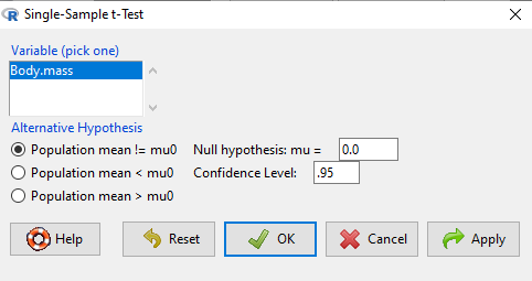
Figure 2. Screenshot Rcmdr single-sample t-test menu.
Type in the value 5.0 in the Null hypothesis: m = u box.
Question 1: Quick! Can you write, in plain old English, the statistical null hypothesis???
Answer 1: For example: No difference between gecko and Anolis lizard mean body mass.
Click OK
The results go to the Output Window.
t.test(lizards$Body.mass, alternative='two.sided', mu=5.0, conf.level=.95)
One Sample t-test
data: lizards$Body.mass
t = -1.5079, df = 7, p-value = 0.1753
alternative hypothesis: true mean is not equal to 5
95 percent confidence interval:
2.668108 5.515892
sample estimates:
mean of x 4.092
end of R output
Let’s identify the parts of the R output from the one sample t-test. R reports the name of the test and identifies
- The
dataset$variableused (lizards$Body.mass). The data set was called “lizards” and the variable was “Body.mass”. R uses the dollar sign ($) to denote the dataset and variable within the data set. - The value of the t test statistic was (t = -1.5079). It is negative because the sample mean was less than the population mean — you should be able to verify this!
- The degrees of freedom, df = 7
- The p-value = 0.1753
- 95% confidence interval of the population mean; lower limit = 2.668108, upper limit = 5.515892
- The sample mean = 4.092
Take a step back and review.
Let’s make sure we “get” the logic of the hypothesis testing we have just completed.
Consider the one-sample t-test.
Step 1. Define HO and HA. The null hypothesis might be that a sample mean, , is equal to μ = 5.
The alternate is that the sample mean is not equal to 20.
Where did the value 5 come from? It could be a value from the literature (does the new sample differ from values obtained in another lab?). The point is that the value is known in advance, before the experiment is conducted, and that makes it a one-sample t-test.
One tailed hypothesis or two?
We introduced you to the idea of “tails of a test” (Ch08.4). As you should recall, a null/alternative hypothesis for a two-tailed test may be written as
Null hypothesis

versus the alternative hypothesis

where is the sample mean and is the population mean.
Alternatively, we can write one-tailed tests of null/alternative hypothesis

for the null hypothesis versus the alternative hypothesis

Question 2: Are all possible outcomes of the one-tailed test covered by these two hypotheses?
Answer 2: Yes
Question 3: What was the SEM for this problem?
Answer 3: It would be the sample standard deviation divided by the square root of the sample size.
Step 2. Decide how certain you wish to be (with what probability) that the sample mean is different from μ. As stated previously, in biology, we say that we are willing to be incorrect 5% of the time (Cowles and Davis 1982; Cohen 1994). This means we are likely to correctly reject the null hypothesis 100% – 5% = 95% of the time, which is the definition of statistical power. We do this by setting the Type I error to be 5% (alpha, α = 0.05). The Type I error is the chance that we will reject a null hypothesis, but the true condition in the population we sampled was actually “no difference.”
Step 3. Carry out the calculation of the test statistic. In other words, get the value of t from the equation above by hand, or, if using R (yes!) simply identify the test statistic value from the R output after conducting the one sample t test.
Step 4. Evaluate the result of the test. If the value of the test statistic is greater than the critical value for the test, then you conclude that the chance (the P-value) that the result could be from that population is not likely and you therefore reject the null hypothesis.
Question 4: What is the critical value for a one-sample t-test with df = 7?
Answer 4: From R, we get + 2.365 for the two-tailed test. R code was qt(c(.025), df=7, lower.tail=FALSE)
Hint; you need the table or better, use R
Rcmdr: Distributions → Continuous distributions → t distributions → t quantiles
You also need to know three additional things to answer this question.
- You need to know alpha (α), which we have said generally is set at 5%.
- You also need to know the degrees of freedom (DF) for the test. For a one sample t-test, DF = n – 1, where n is the sample size.
- You also must know whether your test is one or two-tailed.
- You then use the t-distribution (the tables of the t-distribution at the back of your book) to obtain the critical value. Note that if you use R, the actual p-value is returned.
Why learn the equations when I can just do this in R?
Rcmdr does this for you as soon as you click OK. Rcmdr returns the value of the test statistic and the p-value. R does not show you the critical value, but instead returns the probability that your test statistic is as large as it is AND the null hypothesis is true. From our one-sample t-test example, the Rcmdr output. The simple answer is that in order to understand the R output properly you need to know where each item of the output for a particual test comes from and how to interpret it. Thus, the best way is to have the equations available and to understand the algorithmic approach to statistical inference.
And, this is as good of time as any to show you how to skip the RCmdr GUI and go straight to R.
First, create your variables. At the R prompt enter the first variable
liz <- c("G","G","G","G","A","A","A","A")
and then create the second variable
bm <- c(3.186,2.427,4.031,1.995,5.515,5.659,6.739,3.184)
Next, create a data frame. Think of a data frame as another word for worksheet.
lizz <- data.frame(liz,bm)
Verify that entries are correct. At the R prompt type “lizz” wthout the quotes and you should see
lizz
 liz bm
1 G 3.186
2 G 2.427
3 G 4.031
4 G 1.995
5 A 5.515
6 A 5.659
7 A 6.739
8 A 3.184
End of R output
Carry out the t-test by typing at the R prompt the following
t.test(lizz$bm, alternative='two.sided', mu=5, conf.level=.95)
And, like the Rcmdr output we have for the one-sample t-test the following R output
One Sample t-test
data: lizards$Body.mass
t = -1.5079, df = 7, p-value = 0.1753 alternative hypothesis: true mean is not equal to 5
95 percent confidence interval:
2.668108 5.515892
sample estimates:
mean of x
4.092
End of R output
which, as you probably guessed, is the same as what we got from RCmdr.
Question 5: From the R output of the one sample t-test, what was the value of the test statistic?
- -1.5079
- 7
- 0.1753
- 2.668108
- 5.515892
- 4.092
Answer 5: -1.5079
Note 4: BI311 students — On an exam you will be given portions of statistical tables and output from R. Thus you should be able to evaluate statistical inference questions by completing the missing information. For example, if I give you a test statistic value, whether the test is one- or two-tailed, degrees of freedom, and the Type I error rate alpha, you should know that you would need to find the critical value from the appropriate statistical table. On the other hand, if I give you R output, you should know that the p-value and whether it is less than the Type I error rate of alpha would be all that you need to answer the question.
Why fall back on statistical tables? Think of this as a basic skill. In statistics and for some statistical tests, Rcmdr and other software may not provide the information needed to decide that your test statistic is large, and a table in a statistics book is the best way to evaluate the test.
For now, double check Rcmdr by looking up the critical value from the t-table.
Check critical value against our test statistic
Df = 8 – 1 = 7
The test is two-tailed, therefore α(2)
α = 0.05 (note that two-tailed critical value is 2.365. T was equal to 1.51 (since t-distribution is symmetrical, we can ignore the negative sign), which is smaller than 2.365 and so we would agree with Rcmdr — we cannot reject the null hypothesis.
Question 6: From the R output of the one sample t-test, what was the P-value?
- -1.5079
- 7
- 0.1753
- 2.668108
- 5.515892
Answer 6: 0.1753
Question 7: We would reject the null hypothesis
- False
- True
Answer 7: False — p-value, 17.5%, is greater than Type I error of 5%.
Questions
Seven questions, with answers, were provided for you within the text in this chapter. Here’s one more, but without answers.
8. Here’s a small data set for you to try your hand at the one-sample t-test and Rcmdr. The dataset contains cell counts, five counts of the numbers of beads in a liquid with an automated cell counter (Scepter, Millipore USA). The true value is 200,000 beads per milliliter fluid; the manufacturer claims that the Scepter is accurate within 15%. Does the data conform to the expectations of the manufacturer? Write a hypothesis then test your hypothesis with the one-sample t-test. Here’s the data.
| scepter |
| 258900 |
| 230300 |
| 107700 |
| 152000 |
| 136400 |
Quiz Chapter 8.5
One sample t-test
Chapter 8 contents
8.1 – The null and alternative hypotheses
Introduction
Classical statistical parametric tests — t-test (one sample t-test, independent sample-t-test), analysis of variance (ANOVA), correlation, and linear regression— and nonparametric tests like  (chi-square: goodness of fit and contingency table), share several features that we need to understand. It’s natural to see all the details as if they are specific to each test, but there’s a theme that binds all of the classical statistical inference in order to make claim of “statistical significance.”
- a calculated test statistic
- degrees of freedom associated with the calculation of the test statistic
- a probability value or p-value which is associated with the test statistic, assuming a null hypothesis is “true” in the population from which we sample.
- Recall from our previous discussion (Chapter 8.2) that this is not strictly the interpretation of p-value, but a short-hand for how likely the data fit the null hypothesis. P-value alone can’t tell us about “truth.”
- in the event we reject the null hypothesis, we provisionally accept the alternative hypothesis.
Statistical Inference in the NHST Framework
By inference we mean to imply some formal process by which a conclusion is reached from data analysis of outcomes of an experiment. The process at its best leads to conclusions based on evidence. In statistics, evidence comes about from the careful and reasoned application of statistical procedures and the evaluation of probability (Abelson 1995).
Formally, statistics is rich in inference process (Bzdok et al, 2018). We begin by defining the classical frequentist, aka Neyman-Pearson approach, to inference, which involves the pairing of two kinds of statistical hypotheses: the null hypothesis (HO) and the alternative hypothesis (HA). The null hypothesis assumes that any observed difference between the groups are the results of random chance (introduced in Ch 2.3 – A brief history of (bio)statistics ), where “random chance” implies that outcomes occur without order or pattern (Eagle 2021). Whether we reject or accept the null hypothesis — a short-hand for the more appropriate “provisionally reject” in light of the humility that our results may reflect a rare sampling event — based on the outcome of our statistical inference, the inference is evaluated against a decision criterion (cf discussion in Christiansen 2005), a fixed statistical significance level (Lehmann 1992). Significance level refers to the setting of a p-value threshold before testing is done. The threshold is often set to Type I error of 5% (Cowles & Davis 1982), but researchers should always consider whether this threshold is appropriate for their work (Benjamin et al 2017).
This inference process is referred to as Null Hypothesis Significance Testing, NHST. Additionally, a probability value will be obtained for the test outcome or test statistic value. In the Fisherian likelihood tradition, the magnitude of this statistic value can be associated with a probability value, the p-value, of how likely the result is given the null hypothesis is “true.” (Again, keep in mind that this is not strictly the interpretation of p-value, it’s a short-hand for how likely the data fit the null hypothesis. P-value alone can’t tell us about “truth”, per our discussion, Chapter 8.2.)
Note 1: About reporting p-values, -logP. A Google search will likely reveal “logP,” which is a measure in chemistry. In contrast, “-logP” pertains to how to report p-values in statistics. P-values are traditionally reported as a decimal, like 0.000134, in the closed (set) interval (0,1) — p-values can never be exactly zero or one. The smaller the value, the less the chance our data agree with the null prediction. Small numbers like this can be confusing, particularly if many p-values are reported, like in many genomics works, eg, GWAS studies. In the past, small p-values would be reported as “less than,” eg, < 0.001. This was done in part because of the misleading impression of precision that many significant figures can represent (see discussion in Lang and Altman 2014).
-logP is an alternative, particularly for GWAS studies where the significance level may be much smaller than 5%. Thus, instead of reporting vanishingly small p-values, studies may report the negative log10 p-value, or -logP. Instead of small numbers, large numbers are reported, the larger, the more against the null hypothesis. Thus, our p-value becomes 3.87 -logP.
R code
-1*log(0.000134,10)
[1] 3.872895
Why log10 and not some other base transform? Just that log10 is convenience — powers of 10.
The antilog of 3.87 returns our p-value
> 10^(-1*3.872895)
[1] 0.0001340001
For convenience, a partial p-value -logP transform table
| P-value | -logP |
| 0.1 | 1 |
| 0.01 | 2 |
| 0.001 | 3 |
| 0.0001 | 4 |
On your own, complete the table up to -logP 5 – 10. See Question 7 below.
NHST Workflow
We presented in the introduction to Chapter 8 without discussion a simple flow chart to illustrate the process of decision (Fig 1, Chapter 8). Here, we repeat the flow chart diagram and follow with descriptions of the elements.
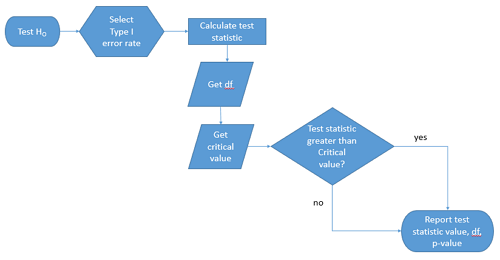
Figure 1. Flow chart of inductive statistical reasoning.
What’s missing from the flow chart is the very necessary caveat that interpretation of the null hypothesis is associated with two kinds of error, Type I error and Type II error. These points and others are discussed in the following sections.
We start with the hypothesis statements. For illustration we discuss hypotheses in terms of comparisons involving just two groups, also called two sample tests. One sample tests in contrast refer to scenarios where you compare a sample statistic to a population value. Extending these concepts to more than two samples is straightforward, but we leave that discussion to Chapters 12 – 18.
Null hypothesis
By far the most common application of the null hypothesis testing paradigm involves the comparisons of different treatment groups on some outcome variable. These kinds of null hypotheses are the subject of Chapters 8 through 12.
The Null hypothesis (HO) is a statement about the comparisons, eg, between a sample statistic and the population, or between two treatment groups. The former is referred to as a one tailed test whereas the latter is called a two-tailed test. The null hypothesis is typically “no statistical difference” between the comparisons.
For example, a one sample, two tailed null hypothesis.

and we read it as “there is no statistical difference between our sample mean and the population mean.” For the more likely case in which no population mean is available, we provide another example, a two sample, two tailed null hypothesis.

Here, we read the statement as “there is no difference between our two sample means.” Equivalently, we interpret the statement as both sample means estimate the same population mean.

Under the Neyman-Pearson approach to inference we have two hypotheses: the null hypothesis and the alternative hypothesis. The hull hypothesis was defined above.
Note 2: Tails of a test are discussed further in chapter 8.4.
Alternative hypothesis
Alternative hypothesis (HA): If we conclude that the null hypothesis is false, or rather and more precisely, we find that we provisionally fail to reject the null hypothesis, then we provisionally accept the alternative hypothesis. The view then is that something other than random chance has influenced the sample observations. Note that the pairing of null and alternative hypotheses covers all possible outcomes. We do not, however, say that we have evidence for the alternative hypothesis under this statistical regimen (Abelson 1995). We tested the null hypothesis, not the alternative hypothesis. Thus, it is incorrect to write that, having found a statistical difference between two drug treatments, say aspirin and acetaminophen for relief of migraine symptoms, it is not correct to conclude that we have proven the case that acetaminophen improves improves symptoms of migraine sufferers.
For the one sample, two tailed null hypothesis, the alternative hypothesis is

and we read it as “there is a statistical difference between our sample mean and the population mean.” For the two sample, two tailed null hypothesis, the alternative hypothesis would be

and we read it as “there is a statistical difference between our two sample means.”
Alternative hypothesis often may be the research hypothesis.
It may be helpful to distinguish between technical hypotheses, scientific hypothesis, or the equality of different kinds of treatments. Tests of technical hypotheses include the testing of statistical assumptions like normality assumption (see Chapter 13.3) and homogeneity of variances (Chapter 13.4). The results of inferences about technical hypotheses are used by the statistician to justify selection of parametric statistical tests (Chapter 13). The testing of some scientific hypothesis like whether or not there is a positive link between lifespan and insulin-like growth factor levels in humans (Fontana et al 2008), like the link between lifespan and IGFs in other organisms (Holtzenberger et al 2003), can be further advanced by considering multiple hypotheses and a test of nested hypotheses and evaluated either in Bayesian or likelihood approaches (Chapter 16 and Chapter 17). The advantage of the Bayesian approach is that it returns evidence for or against this hypothesis: if the posterior probability is greater than the prior probability, we can we say that we have evidence for the hypothesis. This is very appealing — the challenge is that the prior probability is inherently subjective (Chapter 6.4), limited by the amount and quality of existing information pertaining to the hypothesis (Prelec 2004).
Note 3: In Bayesian statistics, hypotheses and their parameters are treated as random variables and we can assign them probabilities. The prior probability is your initial belief about the likelihood of an event before adding new data. The posterior probability is the updated probability after new data has been added. Thus, the posterior combines your prior belief with the new information (the likelihood).
In the frequentis approach, the null hypothesis is no difference (no effect); in the Bayesian context, we’d treat this as a point estimate of zero and have to assign it a probability. In the absence of empirical evidence, one option is to set the probability as 50%, equal prior odds. Use of the spike and slab prior is likely a better approach. There’s a lot of work on these points; I refer interested readers to Campbell and Gustafson (2024) for additional readings and discussion.
How to interpret the results of a statistical test.
Any number of statistical tests may be used to calculate the value of the test statistic. For example, a one sample t-test may be used to evaluate the difference between the sample mean and the population mean (Chapter 8.5) or the independent sample t-test may be used to evaluate the difference between means of the control group and the treatment group (Chapter 10). The test statistic is the particular value of the outcome of our evaluation of the hypothesis and it is associated with the p-value. In other words, given the assumption of a particular probability distribution, in this case the t-distribution, we can associate a probability, the p-value, that we observed the particular value of the test statistic and the null hypothesis is true in the reference population.
By convention, we determine statistical significance (Cox 1982; Whitley & Ball 2002) by assigning ahead of time a decision probability called the Type I error rate, often given the symbol α (alpha). The practice is to look up the critical value that corresponds to the outcome of the test with degrees of freedom like your experiment and at the Type I error rate that you selected. The Degrees of Freedom (DF, df, or sometimes noted by the symbol v), are the number of independent pieces of information available to you. Knowing the degrees of freedom is a crucial piece of information for making the correct tests. Each statistical test has a specific formula for obtaining the independent information available for the statistical test. We first were introduced to DF when we calculated the sample variance with the Bessel correction, n – 1, instead of dividing through by n. With the df in hand, the value of the test statistic is compared to the critical value for our null hypothesis. If the test statistic is smaller than the critical value, we fail to reject the null hypothesis. If, however, the test statistic is greater than the critical value, then we provisionally reject the null hypothesis. This critical value comes from a probability distribution appropriate for the kind of sampling and properties of the measurement we are using. In other words, the rejection criterion for the null hypothesis is set to a critical value, which corresponds to a known probability, the Type I error rate.
Before proceeding with yet another interpretation, and hopefully less technical discussion about test statistics and critical values, we need to discuss the two types of statistical errors. The Type I error rate is the statistical error assigned to the probability that we may reject a null hypothesis as a result of our evaluation of our data when in fact in the reference population, the null hypothesis is, in fact, true. In Biology we generally use Type I error α = 0.05 level of significance. We say that the probability of obtaining the observed value AND HO is true is 1 in 20 (5%) if α = 0.05. Put another way, we are willing to reject the Null Hypothesis when there is only a 5% chance that the observations could occur and the Null hypothesis is still true. Our test statistic is associated with the p-value; the critical value is associated with the Type I error rate. If and only if the test statistic value equals the critical value will the p-value equal the Type I error rate.
The second error type associated with hypothesis testing is, β, the Type II statistical error rate. This is the case where we accept or fail to reject a null hypothesis based on our data, but in the reference population, the situation is that indeed, the null hypothesis is actually false. We must also keep in mind that, as we evaluate the p-value relative to the magnitude of the Type I error rate, and if we reject the null hypothesis, we still do not say that we have evidence for the alternative hypothesis.
Thus, we end with a concept that may take you a while to come to terms with — there are four, not two possible outcomes of an experiment.
Outcomes of an experiment
What are the possible outcomes of a comparative experiment\? We have two treatments, one in which subjects are given a treatment and the other, subjects receive a placebo. Subjects are followed and an outcome is measured. We calculate the descriptive statistics aka summary statistics, means, standard deviations, and perhaps other statistics, and then ask whether there is a difference between the statistics for the groups. So, two possible outcomes of the experiment, correct\? If the treatment has no effect, then we would expect the two groups to have roughly the same values for means, etc., in other words, any difference between the groups is due to chance fluctuations in the measurements and not because of any systematic effect due to the treatment received. Conversely, then if there is a difference due to the treatment, we expect to see a large enough difference in the statistics so that we would notice the systematic effect due to the treatment.
Actually, there are four, not two, possible outcomes of an experiment, just as there were four and not two conclusions about the results of a clinical assay. The four possible outcomes of a test of a statistical null hypothesis are illustrated in Table 1.
Table 1. When conducting hypothesis testing, four outcomes are possible.
| HO in the population | |||
| True | False | ||
| Result of statistical test | Reject HO | Type I error with probability equal to
α (alpha) |
Correct decision, with probability equal to
1 – β (1 – beta) |
| Fail to reject the HO | Correct decision with probability equal to
1 – α (1 – alpha) |
Type II error with probability equal to
β (beta) |
|
In the actual population, a thing happens or it doesn’t. The null hypothesis is either true or it is not. But we don’t have access to the reference population, we don’t have a census. In other words, there is truth, but we don’t have access to the truth. We can weight, assigned as a probability or p-value, our decisions by how likely our results are given the assumption that the truth is indeed “no difference.”
If you recall, we’ve seen a table like Table 1 before in our discussion of conditional probability and risk analysis (Chapter 7.3). We made the point that statistical inference and the interpretation of clinical tests are similar (Browner and Newman 1987). From the perspective of ordering a diagnostic test, the proper null hypothesis would be the patient does not have the disease. For your review, here’s that table (Table 2).
Table 2. Interpretations of results of a diagnostic or clinical test.
| Does the person have the disease\? | |||
| Yes | No | ||
| Result of the diagnostic test |
Positive | sensitivity of the test (a) | False positive (b) |
| Negative | False negative (c) | specificity of the test (d) | |
Thus, a positive diagnostic test result is interpreted as rejecting the null hypothesis. If the person actually does not have the disease, then the positive diagnostic test is a false positive.
Questions
- Match the corresponding entries in the two tables. For example, which outcome from the inference/hypothesis table matches specificity of the test \?
- Find three sources on the web for definitions of the p-value. Write out these definitions in your notes and compare them.
- In your own words distinguish between the test statistic and the critical value.
- All of our discussions have been about testing the null hypothesis, about accepting or rejecting, provisionally, the null hypothesis.
- What are the p-values for -logP of 5, 6, 7, 8, 9, and 10 \? Complete the p-value -logP transform table.
- Instead of log10 transform, create a similar table but for negative natural log transform. Which is more convenient? Hint:
log(x, base=exp(1))
Quiz Chapter 8.1
The null and alternate hypothesis