3.4 – Estimating parameters
Introduction.
What you will find on this page. Definitions for constants, variables, and parameters as used in data analytics. Statistical bias and the concept of unbiased estimators are discussed. The different types of error are introduced along with definitions of accuracy and precision. Statistics used to quantify error are presented in the next section, Chapter 3.4.
Estimating parameters.
Parameters belong to populations; they are fixed but unknown. Parameters are characteristics of populations: the typical average height and weight of five year old children; What is the normal range of values for height and weight of five year old children; average and range of gene expression of TP53 in epithelial lung cells of 50 year old non-smoking humans; etc. Because we generally do not have at our disposal surveys — census — of entire populations for these characteristics, we sample and calculate descriptive statistics for a subset of individuals from populations: these statistics, the mean height, range of height, etc., are variables. We expect average height, range of height, etc., to change, to vary, from sample to sample. A constant, as the word implies, is not variable and remains unchanged.
We estimate parameters (means, variances) from samples of observations from a population. Intuitively then, our estimates are only as good as how representative of the population the sample is. Statistics allows us to be more precise: we can define “how good” our estimates are by asking about, and quantifying, the accuracy and precision of our estimates.
Notwithstanding the notion of “personalized medicine,” our goal in science is to understand cause and effect among sets of observations on samples from a population. We ask, what is the link between lung cancer and smoking? We know that smoking tobacco cigarettes increases risk of cancer, but not everyone who smokes will get cancer (Pesch et al., 2012). Tumorigenic risk is in part mediated by heredity (cf. Trifiletti et al 2017). That’s one way we run into problems in statistics: the biological phenomenon is complicated in ways we are not yet aware of, and thus samples drawn from populations are heterogeneous. Put another way, we think there is one population, but there may be many distinct populations. By chance, repeated samples drawn from the population include individuals with different risk associated with heredity.
As an aside, this is precisely why the concept of personalized medicine is important. Medical researchers have learned that some people with breast cancer respond to treatment with trastuzumab, a monoclonal antibody, but others do not (review in Valabrega et al 2007). Responders have more copies of a gene, copy number variation, for an EGF-like receptor called HER2. In contrast, non-responders to trastuzumab have fewer copies of this receptor (and are said to be HER2-negative in an antibody test for HER2). Thus, we speak about people with breast cancer as if the disease is the same, and from a statistical point of view, we would assume that individuals with breast cancer are of the same population. But they are not — and so the treatment fails for some, but works for others. In this example, we have a mechanism or cause to explain why some do not respond; their breast cancer is not associated with increased copy numbers of HER2. And so in studies with breast cancer, statisticians may account for differences in HER2 status. Note: Fewer than 30% of breast cancer may have over-expression of HER2, (Bilous et al. 2003).
Clearly, HER2 status would be used by statisticians when drawing samples from population, and we would not mistake samples. But, in many other situations we are not aware of any differences and so we assume our samples come from the same population. Note that even with imperfect knowledge about samples, experimental design is intended to help mediate heterogeneous samples. For example, this is why treatment controls need to be used, or case controls are included in studies.
Random assignment to groups also is an attempt to control for unknowns: if random, then all treatment groups will likely include representatives of the numerous co-factors that contribute to risk.
Statisticians have an additional, technical burden: there are often a variety of ways (algorithms) to describe or make inferences about samples, and they are not equally capable of giving us “truth.” Estimates of a parameter are not going to be exactly the true value of the parameter! This is the problem of identifying unbiased ways to estimate parameters. In statistics, bias quantifies whether an algorithm to calculate a particular statistic (e.g., the mean or variance), is consistently too low or too high.
Random sampling.
Random sampling from the population is likely to be our best procedure for obtaining representative samples, but it is not foolproof (we’ll return to situations where random sampling fails to provide adequate samples of populations in Chapter 5.5 Importance of randomization in experimental design). However, a second concern is how to calculate the mean, how to calculate the variance. In the section on Descriptive Statistics (Chapter 3.2), we presented how to calculate the arithmetic mean — the simple average — but also introduced you to other calculations for the middle (e.g., median, geometric mean, harmonic mean). How to know which “middle” is correct?
Statisticians use the concept of bias — the simple arithmetic mean is an unbiased estimator of the population parameter, but a correction needs to be made to the calculation of sample variance to remove bias. Bias implies that the estimator systematically misses the target in some way. Good or “best” parameter estimates are, on average, going to be close to the actual parameter if we collected many samples of the population (this will depend on the sample size and the variability of the data). Earlier we introduced Bessel’s correction to the sample variance, divide the sum of squares by n – 1 and not N as we did for the population variance, so that it is an unbiased estimator of the sample variance. Thus, statisticians have worked out how well their statistical equations work as estimators; concepts of expected values or the expectation are used to evaluate how well an estimator works. In statistics, the expected value of a statistic is calculated by multiplying each of the possible outcomes by the likelihood each outcome will occur and then summing all of those values..
We need to add a bit more to our discussion about measurement and estimation.
Types of error.
To measure is to assign a number to something, a variable. Measurements can have multiple levels, but are of the four data types: nominal, ordinal, interval scale, and ratio scale. Nominal and ordinal types are categorical or qualitative; interval and ratio are continuous or quantitative. Errors in measurement represent differences between what is observed and recorded compared with the true value, i.e., the actual population value. With respect to measurement we distinguish between random errors and systematic errors. Random errors occur by chance, and are thus expected to vary from one measurement instance from another. Random error may lead to measures larger or smaller than the true value. Systematic errors are of a kind that can be attributed to failures of an experimental design or instrument.
Accuracy is reflected in the question: how close to the true value is our measure? Accuracy is distinct from precision, the concept of how clustered together are repeated values for the same measurement. All measurement has associated error, which may be divided into two kinds: random error and systematic error.
We tend to think of error in terms of mistakes, mistakes by us or as failure of the measurement process. However, in biology research, that is too restrictive of a meaning for error. First, experimental error occurs when the estimates derived from the samples — sample mean, sample variance — differ from the population parameters — population mean, population variance. Second, error in biology ranges from mistakes in data collection to real differences among individuals for a characteristic. The latter source, error among individuals, is of course, not a mistake, but rather, it’s the “very spice of life” (Cowper 1845). We’ll leave the study of individual differences, biological error, for later. This section is concerned with error in the sense of mistakes.
Random error includes things like chance error in an instrument leading to different repeat measures of the same thing and to the reality that individual differences exist for most biological traits. We minimize the effects of this kind of error by randomizing: we randomly select samples from populations; we randomly assign samples to treatment groups. Random error can make it hard to differentiate treatment effects. Random error decreases precision, the repeatability of measures. At worse, random error is conservative — it tends to mean we miss group differences, we conclude that the treatment (e.g., aspirin analgesics) has no effect on the condition (e.g., migraines). This kind of error is referred to as a Type II error (Chapter 8).
The experimental design remedy for random error is to increase sample size, a key conclusion drawn from power analysis on experiments, discussed in Chapter 11. The other type of error, systematic error, a type of bias, is more in line with the idea of errors being synonymous with mistakes. Uncalibrated instruments yield incorrect measures. And these kinds of errors lead us to make errors that can be more problematic. An example? Back in the early 1990s when I started research on whole animal metabolic rates (e.g., Dohm et al 1994, Beck et al 1995), we routinely set baseline carbon dioxide, CO2, levels to 0.035% of volume of dry air (350 ppm, parts per million), which reflected ambient levels of CO2 at the time (see Figure 4 in Chapter 4.6).
#NOAA monthly data from Mauna Loa Observatory
co2.1994 <- c(358.22, 358.98, 359.91, 361.32, 361.68, 360.80, 359.39, 357.42, 355.63, 356.09, 357.56, 358.87)
You are probably aware, today, background CO2 have increased considerably even since the 1980s. Data for 2021 (average 420 ppm — reporting just 2 significant figures) are provided below
co2.2021 <- c(415.49, 416.72, 417.61, 419.01, 419.09, 418.93, 416.9, 414.42, 413.26, 413.9, 414.97, 416.67)
source: Global Monitoring Lab, NOAA
Thus, if I naively compared rates of CO2 produced by an animal at rest,  , measured today against the data I gathered back in the 1990s without account for the change in background CO2 in my analysis, I will have committed a systematic error: values of on animals would be systematically higher than values for 1988 when I apply a baseline correction.
Examples of error.
One under-reported cost of next-generation sequencing technologies is that base calls, the process of assigning a nucleotide base to chromatogram peaks has more errors than traditional Sanger-based sequencing methods (Fox et al 2014). In “next-generation-sequencing” (NGS) methods, individual DNA fragments are assigned sequences, whereas Sanger methods took the average sequence of a collection of DNA fragments; thus, in principle, NGS methods should be able to characterize variation of mixtures of sequences in ways not available to traditional sequencing approaches. However, artifacts introduced in sample preparation and PCR amplification lead to base calling errors (Fox et al 2014).
Gene expression levels will differ among tissue types, thus mixed samples from different tissues will misrepresent gene expression levels.
Measurement of energy expenditure, oxygen uptake and carbon dioxide release by an organism, have long been sources of study in ecology and other disciplines. A classic measure is called basal metabolic rate, measured as the rate of oxygen consumption of an endothermic animal, post-absorptive (i.e., not digesting food), at rest but not sleeping, while the animal is contained within a thermal-neutral environment (Blaxter 1989).
Accuracy and precision.
Two properties of measurement are the accuracy of the measure and its precision. Accuracy is defined as the closeness of a measured value to its true value. Precision refers to the closeness of a second measure to the first, to the closeness of a third measure to the first and second, and so on. Precision refers to repeatability of measurement. We suggested use of the coefficient of variation, defined with examples in Chapter 3.2, as a way to quantify precision.
Consider the accuracy and precision of three volumetric pipettors: p1000, which has a nominal range between 100 and 1000 μL (microliters); p200, which has a range between 20 and 200 μL; p100, which has a range between 10 and 100 μL. Which of these three pipettors do you think would have the best accuracy and precision for dispensing 100 μL? We can test pipettors by measuring the mass of distilled water dispensed by the pipettor on an analytical balance. For 100 μL of distilled water at standard temperature and pressure conditions, the mass of the water would be 0.100 grams. The results are shown in the table, and a dot plot is shown in the figure to help us see the numbers.
Table 1. Mass (grams) of 100 μL of distilled water dispensed by three volumetric pipettors*
| p1000 | p200 | p100 | |
| 0.113 | 0.100 | 0.101 | |
| 0.114 | 0.100 | 0.100 | |
| 0.113 | 0.100 | 0.100 | |
| 0.115 | 0.099 | 0.101 | |
| 0.113 | 0.100 | 0.101 | |
| 0.112 | 0.100 | 0.100 | |
| 0.113 | 0.100 | 0.100 | |
| 0.111 | 0.100 | 0.100 | |
| 0.114 | 0.101 | 0.101 | |
| 0.112 | 0.100 | 0.100 | |
| mean: | 0.113 | 0.100 | 0.1004 |
| standard deviation: | 0.0012 | 0.0005 | 0.0005 |
*Temperature 21.5 °C, barometric pressure 76.28 cm mercury (elevation 52 meters). Data presented in Table 1 were not corrected to standard temperature or pressure.
Here is the code for the R run; assuming that you have started R commander, then copy and paste each line into the R Commander script window; if not, enter the script one line at a time in the R console. Recall that the hashtag, #, is used to add comment lines.
Note 1: A reminder: Don’t include the last two rows from Table 1 in your data set; these contain descriptive statistics and are not your data.
#create the variables
p1000 <- c(0.113, 0.114, 0.113, 0.115, 0.113, 0.112, 0.113, 0.111, 0.114, 0.112)
p100 <- c(0.101, 0.1, 0.1, 0.101, 0.101, 0.1, 0.1, 0.1, 0.101, 0.1)
p200 <- c(0.1, 0.1, 0.1, 0.099, 0.1, 0.1, 0.1, 0.1, 0.101, 0.1)
#create a data frame
pipet <- data.frame(p100,p200,p1000)
attach(pipet)
#stack the data
stackPipet <- stack(pipet[, c("p100","p200","p1000")])
#Add variable names
names(stackPipet) <- c("mass", "pipet")
#create the dot plot
with(stackPipet, RcmdrMisc::Dotplot(mass, by=pipet, bin=FALSE))
From Table 1 we see that the means for the p100 and p200 were both close to the target mass of 0.1 g. The mean for the p1000, however, was higher than the target mass of 0.1 g. A dot plot is a good way to display measurements (Fig. 1).
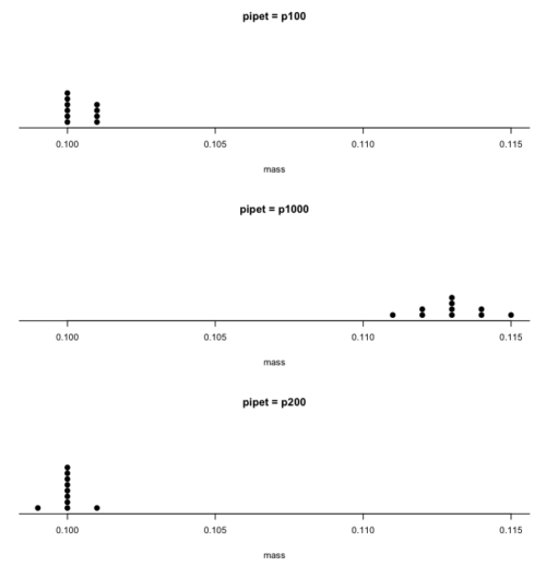
Figure 1. Dot plot of pipet results.
Note 2: Dotplot() is part of the RcmdrMisc package; if you are using the Rcmdr script window (please do!), then the functions in RcmdrMisc are already available and you wouldn’t need to use RcmdrMisc:: (package name plus double-colon operator) to call the Dotplot() function (more properly, referred to as namespaces). Thus, with(stackPipet, Dotplot(mass, by=pipet, bin=FALSE)) would work perfectly well within the Rcmdr script window.
From the dot plot we can quickly see that the p1000 was both inaccurate (the data fall well above the true value), and lacked precision (the values were spread about the mean value). The other two pipettors showed accuracy and looked to be similar in precision, although only two of ten values for the p200 were off target compared to four of ten values for the p100. Thus, we would conclude that the p200 was best at dispensing 100 microliters of water.
In the next chapter we apply statistics to estimate our confidence in this conclusion. In contrast to measurement, estimation implies calculation of a value. In statistics, estimates may be a point, e.g., a value of a collection of data, or an interval, e.g., a confidence interval.
Summary.
This is your first introduction into the concept of experimental design, as defined by statisticians! One of the key tasks for a statistical analyst is to have an appreciation for measurement accuracy and precision as established in the experiment. Precise and accurate measurement levels determine how well questions about the experiment can be answered. At one extreme, if a measure is imprecise, but accurate, then it will be challenging to quantify differences between a control group and a treatment group. At the other extreme, if the measure is precise, but inaccurate, the danger would be differences between the treatment and control group may be more likely, even when the groups are truly not different!
Questions.
- List the types of error in measuring mRNA expression levels on a gene for a sampling of cells from biopsy of normal tissue and a biopsy of a tumor. Assume use of NEXGEN methods for measuring gene expression. Distinguish between technical errors and biological errors.
- If confidence interval are useful for estimating accuracy, what statistic do we call to quantify precision?
Quiz Chapter 3.4
Estimating parameters
Chapter 3 contents
2.6 – Statistical reasoning
How statistical reasoning helps us spot and reduce bias.
.
So far in the course we have talked about statistical reasoning. Statistical reasoning as part of the critical thinking tool kit. What this should mean for you in practice is that we will be developing and enhancing your critical thinking skill set. Here, we’ll define our terms and place statistical reasoning in context.
Critical thinking.
.
What do I mean by critical thinking? You’ll find various definitions and discussions, but the Wikipedia entry on the subject seems as good a start as anything else I have heard or read:
“Critical thinking is a way of deciding whether a claim is always true, sometimes true, partly true, or false” (5 August 2013, http://en.wikipedia.org/wiki/Critical_thinking).
Which raises the question, what is truth (false)? And what about the frequency qualifiers “always,” “sometimes,” “partly”? This hints at one of the strengths of science; “Truth in science … is never final, and what is accepted as fact today may be modified or even discarded tomorrow” (p. 2, National Academy of Science 1999). Scientists extend and even correct the work of their predecessors.
Critical thinking has many definitions, but they coalesce broadly as the search for rational justification — arguments and decisions based on reason not emotion — given sets of facts. We’ll define facts as assertions about the world that are verifiably true. Related to facts, we define evidence as collection of facts used to infer an assertion or belief is objectively true. Objectivity holds independently of the observer. In practice, critical thinking can be improved by identifying and developing certain skill sets, from deductive reasoning to use of a statistical toolkit, although skills alone do not necessarily lead to sound critical thinking (Bailin 2002). Emphasis on the importance of statistical reasoning, for example in the Evidence-Based Medicine (EBM) approach, is now well established. EBM is an expansive concept, but includes the philosophy that decisions in medicine and health care should be based on evidence (results) from well designed and executed research. More generally, much has been written on the subject. My purpose here is to sell you just a bit that you will learn more than formulas and statistical tests in this course; if we do this right you will improve your critical thinking skills.
And the tool kit for critical thinking? Science has the scientific method to offer. In turn, by adopting statistical reasoning approaches you will be more cognizant of whether or not you are indeed engaged in critical thinking about your work.
A working checklist for critical evaluation of a project
- “All sides” of the problem are fairly represented
- Authority is not synonymous with empirical truth: trust, but verify
- Correlation (association) may or may not infer causation
- Do conflicts of interest compromise conclusions?
In other words, identify and rigorously consider assumptions made to reach conclusions, evidence given in support of conclusions, and considerations of bias held by the researcher. The “all sides” part requires judgement — not all sides of a research question are equally valid; the point about “fair” representation requires that opposing arguments are actually held by others and not simply a “”straw man” characterization of of a position held by no one.
Rigid adherence to “how to do science checklist” is likely to be wanting and thus practicing and successful scientists show more flexibility. And, the list is certainly incomplete because it presumes observations and data collection are from a reliable, unbiased source. Before proceeding with how statistics informs our critical thinking in science, let’s illustrate bias.
Bias everywhere.
.
Bias is defined as any tendency that may hamper our ability to answer a question without prejudice (Pannucci and Wilkins 2010). Although we tend to think of ourselves as highly rational (Note 1), psychologists have documented, named numerous, and in some cases, highly specific kinds of cognitive biases we may have about “real world data” that may impair our judgment about results of experiments.
Note 1. A handful of Nobel prizes were awarded over evidence and theory on just how unrational we are, see Simon (1978), Kahneman (2002), and Thaler (2017, whose views were immortalized in the movie The Big Short).
At its best, application of the scientific method is our best tool kit to help protect our conclusions against bias (Nuzzo 2015), by proper experimental design and possible study biases. A couple of comics from xkcd illustrate.
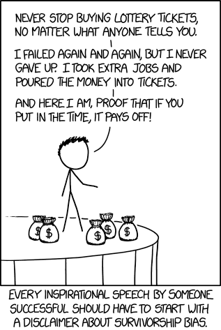
Figure 1. “Survivorship bias,” https://www.xkcd.com/1827/ .
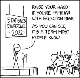
Figure 2. “Selection bias,” https://xkcd.com/2618/ .
Wikipedia lists dozens of named biases which may influence our ability to interpret science:
- confirmation bias, eg, given extraneous information about ancestry or sex, forensic investigators were more likely to assign ancestry or sex of skeletal evidence to group that confirmed the contextual information (Nakhaeizadeh et al 2014).
- congruence bias, a type of confirmation bias, the tendency to test only a favorite or initial hypothesis over consideration of alternative hypotheses.
- observer-expectancy bias, eg, randomized controlled trials of acupuncture often find equivalent responses to real and placebo acupuncture despite both appearing superior to no treatment (Colagiuri and Smith 2012).
- selection bias, the selection of individuals, groups, or data for analysis in such a way that proper randomization is not achieved, eg, mitotic counts (Cree et al 2021) and cell differentials and Figure 2. Selection bias, where the study population is not well-defined or if is, the method by which subjects are recruited favors one kind of subject over another.
- surveillance bias, eg, association between myocarditis and COVID-19 vaccines may be due to increased focus to identify myocarditis (Husby et al 2021).
- survivorship bias, focusing on subjects that passed a selection process as if they represent an entire group, eg, from ecology: rare species more likely to go extinct than abundant species (Lockwood 2003) and Figure 1.
Bias in research may occur at any level, from study design to analysis and publication of results. Bias leads to systematic errors that may favor one outcome over others. Clearly then, bias is something one wants to avoid in science, and most scientists would probably agree strongly that bias is unacceptable. However, bias can creep into projects in many forms.
Particularly pernicious causes of bias are conflicts of interest, with the notable case of a 1990’s set of trials in gene therapy (Wilson 2010). Biased research may be more harmful to science than deliberate misconduct, at least in part because there are, or should be, mechanisms to detect fraud (eg, Marusic et al 2007). If errors in data analysis or management are rare, we can trust the results; if errors are common, systematic, or deliberate falsification, then any conclusions drawn from such work deserves retraction at the very least (cf. discussion in Baggerly and Coombs 2009; see StatCheck project, Nuijten et al 12016).
Bias in research.
.
Bias is not limited to obvious profit seeking or even defense of one’s ideas or reputation. Bias can enter research in subtle ways. Prior to 2000, many post-menopausal women could expect to be placed on hormone replacement therapy (HRT) to manage post-menopausal symptoms and to reduce likelihood of osteoporosis later in life. Moreover, HRT was believed based on research to show protective benefits against heart disease (eg, Nabulsi et al 1993; Grodstein et al 2000). However, other prospective studies that were designed to reduce many sources of bias in patient recruitment (Women’s Health Initiative Study Group 1998), found the opposite: HRT may increase risk of heart disease as well as other diseases (Rossouw et al 2002). Since the 2002 Women’s Health Initiative study report, the costs and benefits of HRT have been furiously debated (Lukes 2008).
The purpose of this chapter, however, is not to exhaustively review sources of bias. Instead, we leave you with a partial list of kinds of bias in clinical trials (from a review by Pannucci and Wilkins 2010).
- Bias during study design, eg, use of subjective measures or poorly designed questionnaires.
- Interviewer bias, for example, if the interviewer is aware of the subject’s condition
- Chronology bias, where the control subjects may not be observed in the same time frame as the treatment subjects
- Citation (reporting) bias, where negative results are not reported
- Confounding, where results may be due to factors not properly controlled that also affect the outcome. An example provided was link between income and health status, which would be confounded by access to health care.
These are but a few of the kinds of bias that even proper research may be influenced by. Solutions are to randomize, to double-blind, and to avoid reporting bias. Controls of sources of bias increase the validity of the research. How experimental design may control for bias is discussed further in Chapter 5.3.
A case study.
.
Stories we hear from the news or from our friends about health or the environment are anecdotal. A basic rule in critical thinking is to distinguish between argument that is built on anecdotal evidence and argument based on scientific evidence. Let’s evaluate the following real-world example.
Airborne® is a leading dietary supplement. Here’s what their website has to say about the product.
“Scientific research confirms that Airborne proprietary formulation with 13 vitamins and minerals plus a blend of health-promoting herbs, does indeed enhance immunity (5 August 2013, http://www.airbornehealth.com/our-story).
This next statement appears in smaller text near the bottom of the page.
“These statements have not been evaluated by the Food and Drug Administration. These products are not intended to diagnose, treat, cure or prevent disease” (5 August 2013, http://www.airbornehealth.com/our-story).
So, in short, how do you evaluate Airborne? The claim is that “scientific research confirms that Airborne … enhance immunity,” and yet, there is a statement that follows that suggests that the claim has not been evaluated by the agency legally responsible in the USA for determining the efficacy of medicine and treatments.
Note 2. “enhance” immunity is a vacuous phrase. Immunity is not a single object. If by immunity we mean resistant to a particular pathogen, this cannot be what the makers literally mean because that would be in violation of the FDA. Yes, deficiencies of vitamin C and other nutrients impair immune function (Carr and Maggini 2017), but there is no evidence to support the claim that Vitamin C supplementation above RDA, recommended dietary allowances, improves resistance. See 2013 Cochrane Review.
Are not these in contradiction? In the USA, supplement manufactures’ need not seek FDA approval. In fact, the U.S. Congress, in it’s passing of the The Dietary Supplement Health and Education Act of 1994 (DSHEA), specified what needs to be reported to the FDA; statements of “enhancing immunity” are lawful, but do not require the supplement manufacture to show evidence that their product provides this support, only that ingredients in the supplement may do so.
Returning to the statements from Airborne Health, how may these statements be interpreted?
- peer-reviewed articles testing Airborne are available
- that experiments were conducted without bias
- and that to “enhance immunity” is something one could measure
Let’s look at #3 first. A search of PubMed (December 2013) for the phrase “enhance immunity” returned 9171 hits. I didn’t look through the more than 9000 articles, but a quick look shows that the term is indeed used in research, but carries a wide range of interpretations. For one paper “enhance immune” response was the result of genetic modifications to T-cells and how they responded to a virus (PMID:24324159).
Adding “vitamin” to the search resulted in just 158 hits in PubMed; none of these are about Airborne (see claim #1 and #2). However, to be fair, go back and look at their statement — notice they are not saying exactly that anyone has studied Airborne (otherwise they’d probably list the papers), just that vitamins and minerals and herbs that are in Airborne have been studied.
Indeed, vitamins A, C, E and minerals like zinc and selenium that are in Airborne are among the 158 papers. To be additionally fair to Airborne, there are indeed many papers investigating benefits (harm) of supplemental vitamins and minerals — and again, being charitable here, what we can say is that results are at best inconsistent (Bjelakovic et al 2014; Comerford 2013).
The manufacturer of Airborne ran into some trouble with the FTC and ended up paying over $20 million US dollars to settle the lawsuit. The one study, not peer-reviewed, of Airborne’s effectiveness cited during these proceedings apparently was sponsored by Airborne’s manufacturer. Airborne was acquired by Schiff Vitamins March 2012 (Bloomberg News). Click here for additional reading about Airborne.
About peer-review.
.
Evaluation of claims made, research reported, and ideas in science are generally expected to be subject to peer-review by knowledgeable persons in the field. Effective peer-review is an important “gatekeeper” in science (Siler et al 2015, Tennant 2018). Proper peer review gives legitimacy to research (Siler et al 2015). The traditional peer review system is a closed system, which includes elements controlled by journal editors and is based on reviewer identify remaining anonymous. The closed peer-review system is not the only option: many have argued for an open review process (eg, Pöschl 2012, Ho et al 2013).
Does the Airborne story meet your definition of bias?
.
Airborne made health claims I about their product; these claims were found by the federal government to be misleading but does not fit into our discussion of bias. Instead, Airborne story fits more with critical thinking: I think it is rather a casual position to say that we should, and do, think critically of news source or the stories our friends tell us about health.
But bias in science occurs too, and can be very difficult to control or completely eliminate.
Learning statistical reasoning will help develop critical thinking skills.
.
In addition to considering sources of bias, ie, can you trust the messenger, thinking about the sets of facts offered to bolster a claim, it helps to evaluate each fact to see if
- The author is really talking about correlation and has not in fact provided evidence of causation
- vs. experiment, which tests “cause” manipulate
X, doesYchange?
- vs. experiment, which tests “cause” manipulate
- Measurement appropriate?
- Direct or indirect
- Unmeasured important (co)variable
Questions.
.
- Write up three learning outcomes for this page. Hint: Point your favorite generative AI to this page and ask for help.
- The xkcd comic in Figure 1 titles calls it survivorship bias. Provide a definition for this kind of bias and describe the effects on conclusions if it is not accounted for.
- Doctors are encouraged to engage in “evidence based medicine,” that is, decisions about care should be based on data. How may confirmatory bias (from the patient’s point of view, from the doctor’s point of view) influence a discussion of “facts” when deciding on a course of medication therapy — between a well-established medication with many known side-effects and a new, recently approved medicine reported to be as effective as the standard treatment.
Quiz Chapter 2.6
Statistical reasoning
Chapter 2 contents
.