11.1 – What is Statistical Power?

Introduction
Two additional possible outcomes to an experiment
Questions
Quiz
Chapter 11 contents

Introduction

Simply put, the power of a statistical test asks the question: do we have enough data to warrant a scientific conclusion, not just a statistical inference. From the NHST approach to statistics, we define two conditions in our analyses, a null hypothesis, H_O, and the alternative hypothesis, H_A. By now you should have a working definition of H_O and H_A (Chapter 8.1). For the two-sided case (Chapter 8.4), H_O would be no statistical difference between two sample means, whereas for H_A, there was a difference between two sample means. Similarly, for one-sided cases, H_O would be one sample mean greater (less) than or equal to the second sample mean, whereas for H_A, one sample mean is less (greater) than the second mean. Together, these two hypotheses cover all possible outcomes of our experiment!

However, when conducting an experiment to test the null hypothesis four, not two outcomes are possible with respect to “truth” (Table 1), which we introduced first in our Risk analysis chapter and again when we introduced statistical inference.

Table 1. Possible outcomes of an experiment

		In the population, H_o was really…
		True	False
Inference:	Fail to reject H_o	Correct decision p = 1 – α	Type II error p = β
Inference:	Reject H_o	Type I error p = α	Correct decision p = 1 – β

We introduced false positives and false negatives in our discussion of risk analysis, and now generalize these concepts to outcomes of any experiment.

(1) We do not reject the null hypothesis, we state that we are 95% (P = 1 – α) confident that we’ve made the correct decision, and in fact, that is the true situation (“correct decision”). As before this is a true positive.

For example, mean acetylsalicylic acid concentration in a sample of 200 mg, brand-name aspirin tablets really is the same as generic aspirin.

(2) We reject the null hypothesis, we state there is a 5% chance that we could be wrong (P = 1 – β), and in fact, that is the true situation (“correct decision”). As before this is a true negative.

For example, ephedrine really does raise heart rates in people who have taken the stimulant compared to those who have taken a placebo.

Two additional possible outcomes to an experiment

The other two possible outcomes are not desirable but may occur because we are making inferences about populations from limited information (we conduct tests on samples) and because of random chance influencing our measure.

(3) We do not reject the null hypothesis, but in fact, there was a true difference between the two groups and we have therefore committed a Type II error. As before this is a false negative.

(4) We reject the null hypothesis, but in fact, there was no actual difference between the two groups and we have therefore committed a Type I error. As before this is a false positive.

What can we do about these two possible undesirable outcomes?

We set our Type I error rate α, and, therefore our Type II error rate β before we conduct any tests, and these error rates cover the possibility that we may incorrectly conclude that the null hypothesis is false (α), or we may incorrectly conclude that the null hypothesis is true (β). When might these events happen?

The power of a statistical test is the probability that the test will reject the null hypothesis when the alternative hypothesis is true.

A type I error is committed, by chance alone, when our sample is accidentally obtained from the tail of the distribution, thus our sample appears to be different from the population… Below, we have a possible case that, by chance alone, we could be getting all of our subjects from one end of the distribution (Fig 1).

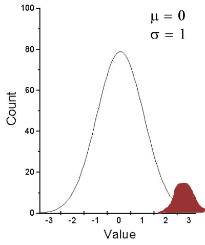
Population sampling from tail of distribution

Figure 1. Population sampling from tail of distribution.

We would likely conclude that our sample mean is different (greater) than the population mean.

A type II error is committed, by chance alone, when our sample is between two different population distributions. The implication for our study is drawn in Figure 2. Instead of our sampling drawn from one population, we may have drawn between two very different populations.

Sample drawn between two populations

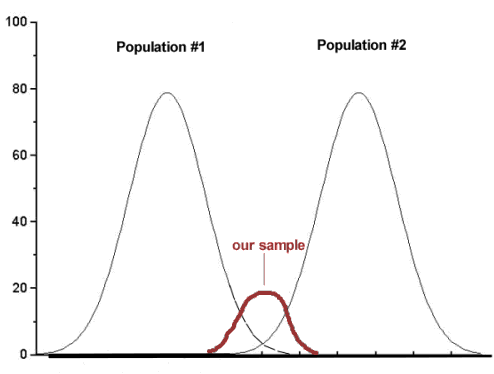
Figure 2. Without us knowing, our sample may come from the extremes of two separate populations.

How did we end up with “the wrong” sample? Recall from our first discussions about Experimental Design how we distinguished between random and haphazard sampling. The key concept was that a program of recruitment of subjects (eg, how to get a sample) must be conducted in such a way that each member of the population has an equal chance of being included in the study. Only then can we be sure that extrinsic factors (things that influence our outcome but are not under our control nor do we study them) are spread over all groups, thus canceling out.

Why do we say we are 95% confident in our estimate (or conclusions)?

(1) Because we can never be 100% certain that by chance alone we haven’t gotten a biased sample (all it takes is a few subjects in some cases to “throw off” our results).

(2) For parametric tests, at least, we assume that we are sampling from a normal population.

Thus, in statistics, we need an additional concept. Not only do we need to know the probability of when we will be wrong (α, β), but we also want to know the probability of when we will be correct when we use a particular statistical test. This latter concept is defined as the power of a test as the probability of correctly rejecting Ho when it is false. Conducting a power analysis before starting the experiment can help answer basic experimental design questions like, how many subjects (experimental units) should my project include? What approximate differences, if any might I expect among the subjects? (Eng 2003; Cohen 1992)

Put another way, power is the likelihood of identifying a significant (important) effect (difference) when one exists. Formally, statistical power is defined as the probability, p = 1 – β, and it is the subject of this chapter.

Questions

Be able to define and distinguish statistical power and statistical inference.

Quiz Chapter 11.1

What is statistical power

Chapter 11 contents

8.1 – The null and alternative hypotheses

Introduction
Statistical Inference in the NHST Framework
NHST Workflow
Null hypothesis
Alternative hypothesis
Alternative hypothesis often may be the research hypothesis
How to interpret the results of a statistical test
Outcomes of an experiment
Questions
Quiz
Chapter 8 contents

Introduction

Classical statistical parametric tests — t-test (one sample t-test, independent sample-t-test), analysis of variance (ANOVA), correlation, and linear regression— and nonparametric tests like $\chi^{2}$ (chi-square: goodness of fit and contingency table ), share several features that we need to understand. It’s natural to see all the details as if they are specific to each test, but there’s a theme that binds all of the classical statistical inference in order to make claim of “statistical significance.”

a calculated test statistic
degrees of freedom associated with the calculation of the test statistic
a probability value or p-value which is associated with the test statistic, assuming a null hypothesis is “true” in the population from which we sample.
- Recall from our previous discussion (Chapter 8.2) that this is not strictly the interpretation of p-value, but a short-hand for how likely the data fit the null hypothesis. P-value alone can’t tell us about “truth.”
in the event we reject the null hypothesis, we provisionally accept the alternative hypothesis.

Statistical Inference in the NHST Framework

By inference we mean to imply some formal process by which a conclusion is reached from data analysis of outcomes of an experiment. The process at its best leads to conclusions based on evidence. In statistics, evidence comes about from the careful and reasoned application of statistical procedures and the evaluation of probability (Abelson 1995).

Formally, statistics is rich in inference process (Bzdok et al, 2018). We begin by defining the classical frequentist, aka Neyman-Pearson approach, to inference, which involves the pairing of two kinds of statistical hypotheses: the null hypothesis (H_O) and the alternative hypothesis (H_A). The null hypothesis assumes that any observed difference between the groups are the results of random chance (introduced in Ch 2.3 – A brief history of (bio)statistics ), where “random chance” implies that outcomes occur without order or pattern (Eagle 2021). Whether we reject or accept the null hypothesis — a short-hand for the more appropriate “provisionally reject” in light of the humility that our results may reflect a rare sampling event — based on the outcome of our statistical inference, the inference is evaluated against a decision criterion (cf discussion in Christiansen 2005), a fixed statistical significance level (Lehmann 1992). Significance level refers to the setting of a p-value threshold before testing is done. The threshold is often set to Type I error of 5% (Cowles & Davis 1982), but researchers should always consider whether this threshold is appropriate for their work (Benjamin et al 2017).

This inference process is referred to as Null Hypothesis Significance Testing, NHST. Additionally, a probability value will be obtained for the test outcome or test statistic value. In the Fisherian likelihood tradition, the magnitude of this statistic value can be associated with a probability value, the p-value, of how likely the result is given the null hypothesis is “true.” (Again, keep in mind that this is not strictly the interpretation of p-value, it’s a short-hand for how likely the data fit the null hypothesis. P-value alone can’t tell us about “truth”, per our discussion, Chapter 8.2.)

Note 1: About reporting p-values, -logP. A Google search will likely reveal “logP,” which is a measure in chemistry. In contrast, “-logP” pertains to how to report p-values in statistics. P-values are traditionally reported as a decimal, like 0.000134, in the closed (set) interval (0,1) — p-values can never be exactly zero or one. The smaller the value, the less the chance our data agree with the null prediction. Small numbers like this can be confusing, particularly if many p-values are reported, like in many genomics works, eg, GWAS studies. In the past, small p-values would be reported as “less than,” eg, < 0.001. This was done in part because of the misleading impression of precision that many significant figures can represent (see discussion in Lang and Altman 2014).

-logP is an alternative, particularly for GWAS studies where the significance level may be much smaller than 5%. Thus, instead of reporting vanishingly small p-values, studies may report the negative log₁₀ p-value, or -logP. Instead of small numbers, large numbers are reported, the larger, the more against the null hypothesis. Thus, our p-value becomes 3.87 -logP.

R code

-1*log(0.000134,10)
[1] 3.872895

Why log₁₀ and not some other base transform? Just that log₁₀ is convenience — powers of 10.

The antilog of 3.87 returns our p-value

> 10^(-1*3.872895)
[1] 0.0001340001

For convenience, a partial p-value -logP transform table

P-value	-logP
0.1	1
0.01	2
0.001	3
0.0001	4

On your own, complete the table up to -logP 5 – 10. See Question 7 below.

NHST Workflow

We presented in the introduction to Chapter 8 without discussion a simple flow chart to illustrate the process of decision (Fig 1, Chapter 8). Here, we repeat the flow chart diagram and follow with descriptions of the elements.

NHST decision flow chart

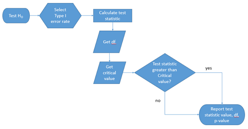
Figure 1. Flow chart of inductive statistical reasoning.

What’s missing from the flow chart is the very necessary caveat that interpretation of the null hypothesis is associated with two kinds of error, Type I error and Type II error. These points and others are discussed in the following sections.

We start with the hypothesis statements. For illustration we discuss hypotheses in terms of comparisons involving just two groups, also called two sample tests. One sample tests in contrast refer to scenarios where you compare a sample statistic to a population value. Extending these concepts to more than two samples is straightforward, but we leave that discussion to Chapters 12 – 18.

Null hypothesis

By far the most common application of the null hypothesis testing paradigm involves the comparisons of different treatment groups on some outcome variable. These kinds of null hypotheses are the subject of Chapters 8 through 12.

The Null hypothesis (H_O) is a statement about the comparisons, eg, between a sample statistic and the population, or between two treatment groups. The former is referred to as a one tailed test whereas the latter is called a two-tailed test. The null hypothesis is typically “no statistical difference” between the comparisons.

For example, a one sample, two tailed null hypothesis.

$\begin{align*} H_{0}: \bar{X} = \mu \end{align*}$

and we read it as “there is no statistical difference between our sample mean and the population mean.” For the more likely case in which no population mean is available, we provide another example, a two sample, two tailed null hypothesis.

$\begin{align*} H_{A}: \bar{X}_{1} = \bar{X}_{2} \end{align*}$

Here, we read the statement as “there is no difference between our two sample means.” Equivalently, we interpret the statement as both sample means estimate the same population mean.

$\begin{align*} H_{A}: \bar{X}_{1} = \bar{X}_{2} = \mu \end{align*}$

Under the Neyman-Pearson approach to inference we have two hypotheses: the null hypothesis and the alternative hypothesis. The hull hypothesis was defined above.

Note 2: Tails of a test are discussed further in chapter 8.4.

Alternative hypothesis

Alternative hypothesis (H_A): If we conclude that the null hypothesis is false, or rather and more precisely, we find that we provisionally fail to reject the null hypothesis, then we provisionally accept the alternative hypothesis. The view then is that something other than random chance has influenced the sample observations. Note that the pairing of null and alternative hypotheses covers all possible outcomes. We do not, however, say that we have evidence for the alternative hypothesis under this statistical regimen (Abelson 1995). We tested the null hypothesis, not the alternative hypothesis. Thus, it is incorrect to write that, having found a statistical difference between two drug treatments, say aspirin and acetaminophen for relief of migraine symptoms, it is not correct to conclude that we have proven the case that acetaminophen improves improves symptoms of migraine sufferers.

For the one sample, two tailed null hypothesis, the alternative hypothesis is

$\begin{align*} H_{A}: \bar{X}\neq \mu \end{align*}$

and we read it as “there is a statistical difference between our sample mean and the population mean.” For the two sample, two tailed null hypothesis, the alternative hypothesis would be

$\begin{align*} H_{A}: \bar{X}_{1}\neq \bar{X}_{2} \end{align*}$

and we read it as “there is a statistical difference between our two sample means.”

Alternative hypothesis often may be the research hypothesis.

It may be helpful to distinguish between technical hypotheses, scientific hypothesis, or the equality of different kinds of treatments. Tests of technical hypotheses include the testing of statistical assumptions like normality assumption (see Chapter 13.3) and homogeneity of variances (Chapter 13.4). The results of inferences about technical hypotheses are used by the statistician to justify selection of parametric statistical tests (Chapter 13). The testing of some scientific hypothesis like whether or not there is a positive link between lifespan and insulin-like growth factor levels in humans (Fontana et al 2008), like the link between lifespan and IGFs in other organisms (Holtzenberger et al 2003), can be further advanced by considering multiple hypotheses and a test of nested hypotheses and evaluated either in Bayesian or likelihood approaches (Chapter 16 and Chapter 17). The advantage of the Bayesian approach is that it returns evidence for or against this hypothesis: if the posterior probability is greater than the prior probability, we can we say that we have evidence for the hypothesis. This is very appealing — the challenge is that the prior probability is inherently subjective (Chapter 6.4), limited by the amount and quality of existing information pertaining to the hypothesis (Prelec 2004).

Note 3: In Bayesian statistics, hypotheses and their parameters are treated as random variables and we can assign them probabilities. The prior probability is your initial belief about the likelihood of an event before adding new data. The posterior probability is the updated probability after new data has been added. Thus, the posterior combines your prior belief with the new information (the likelihood).

In the frequentis approach, the null hypothesis is no difference (no effect); in the Bayesian context, we’d treat this as a point estimate of zero and have to assign it a probability. In the absence of empirical evidence, one option is to set the probability as 50%, equal prior odds. Use of the spike and slab prior is likely a better approach. There’s a lot of work on these points; I refer interested readers to Campbell and Gustafson (2024) for additional readings and discussion.

How to interpret the results of a statistical test.

Any number of statistical tests may be used to calculate the value of the test statistic. For example, a one sample t-test may be used to evaluate the difference between the sample mean and the population mean (Chapter 8.5) or the independent sample t-test may be used to evaluate the difference between means of the control group and the treatment group (Chapter 10). The test statistic is the particular value of the outcome of our evaluation of the hypothesis and it is associated with the p-value. In other words, given the assumption of a particular probability distribution, in this case the t-distribution, we can associate a probability, the p-value, that we observed the particular value of the test statistic and the null hypothesis is true in the reference population.

By convention, we determine statistical significance (Cox 1982; Whitley & Ball 2002) by assigning ahead of time a decision probability called the Type I error rate, often given the symbol α (alpha). The practice is to look up the critical value that corresponds to the outcome of the test with degrees of freedom like your experiment and at the Type I error rate that you selected. The Degrees of Freedom (DF, df, or sometimes noted by the symbol v), are the number of independent pieces of information available to you. Knowing the degrees of freedom is a crucial piece of information for making the correct tests. Each statistical test has a specific formula for obtaining the independent information available for the statistical test. We first were introduced to DF when we calculated the sample variance with the Bessel correction, n – 1, instead of dividing through by n. With the df in hand, the value of the test statistic is compared to the critical value for our null hypothesis. If the test statistic is smaller than the critical value, we fail to reject the null hypothesis. If, however, the test statistic is greater than the critical value, then we provisionally reject the null hypothesis. This critical value comes from a probability distribution appropriate for the kind of sampling and properties of the measurement we are using. In other words, the rejection criterion for the null hypothesis is set to a critical value, which corresponds to a known probability, the Type I error rate.

Before proceeding with yet another interpretation, and hopefully less technical discussion about test statistics and critical values, we need to discuss the two types of statistical errors. The Type I error rate is the statistical error assigned to the probability that we may reject a null hypothesis as a result of our evaluation of our data when in fact in the reference population, the null hypothesis is, in fact, true. In Biology we generally use Type I error α = 0.05 level of significance. We say that the probability of obtaining the observed value AND H_O is true is 1 in 20 (5%) if α = 0.05. Put another way, we are willing to reject the Null Hypothesis when there is only a 5% chance that the observations could occur and the Null hypothesis is still true. Our test statistic is associated with the p-value; the critical value is associated with the Type I error rate. If and only if the test statistic value equals the critical value will the p-value equal the Type I error rate.

The second error type associated with hypothesis testing is, β, the Type II statistical error rate. This is the case where we accept or fail to reject a null hypothesis based on our data, but in the reference population, the situation is that indeed, the null hypothesis is actually false. We must also keep in mind that, as we evaluate the p-value relative to the magnitude of the Type I error rate, and if we reject the null hypothesis, we still do not say that we have evidence for the alternative hypothesis.

Thus, we end with a concept that may take you a while to come to terms with — there are four, not two possible outcomes of an experiment.

Outcomes of an experiment

What are the possible outcomes of a comparative experiment\? We have two treatments, one in which subjects are given a treatment and the other, subjects receive a placebo. Subjects are followed and an outcome is measured. We calculate the descriptive statistics aka summary statistics, means, standard deviations, and perhaps other statistics, and then ask whether there is a difference between the statistics for the groups. So, two possible outcomes of the experiment, correct\? If the treatment has no effect, then we would expect the two groups to have roughly the same values for means, etc., in other words, any difference between the groups is due to chance fluctuations in the measurements and not because of any systematic effect due to the treatment received. Conversely, then if there is a difference due to the treatment, we expect to see a large enough difference in the statistics so that we would notice the systematic effect due to the treatment.

Actually, there are four, not two, possible outcomes of an experiment, just as there were four and not two conclusions about the results of a clinical assay. The four possible outcomes of a test of a statistical null hypothesis are illustrated in Table 1.

Table 1. When conducting hypothesis testing, four outcomes are possible.

		H_O in the population
		True	False
Result of statistical test	Reject H_O	Type I error with probability equal to α (alpha)	Correct decision, with probability equal to 1 – β (1 – beta)
Result of statistical test	Fail to reject the H_O	Correct decision with probability equal to 1 – α (1 – alpha)	Type II error with probability equal to β (beta)

In the actual population, a thing happens or it doesn’t. The null hypothesis is either true or it is not. But we don’t have access to the reference population, we don’t have a census. In other words, there is truth, but we don’t have access to the truth. We can weight, assigned as a probability or p-value, our decisions by how likely our results are given the assumption that the truth is indeed “no difference.”

If you recall, we’ve seen a table like Table 1 before in our discussion of conditional probability and risk analysis (Chapter 7.3). We made the point that statistical inference and the interpretation of clinical tests are similar (Browner and Newman 1987). From the perspective of ordering a diagnostic test, the proper null hypothesis would be the patient does not have the disease. For your review, here’s that table (Table 2).

Table 2. Interpretations of results of a diagnostic or clinical test.

		Does the person have the disease\?
		Yes	No
Result of the diagnostic test	Positive	sensitivity of the test (a)	False positive (b)
Result of the diagnostic test	Negative	False negative (c)	specificity of the test (d)

Thus, a positive diagnostic test result is interpreted as rejecting the null hypothesis. If the person actually does not have the disease, then the positive diagnostic test is a false positive.

Questions

Match the corresponding entries in the two tables. For example, which outcome from the inference/hypothesis table matches specificity of the test \?
Find three sources on the web for definitions of the p-value. Write out these definitions in your notes and compare them.
In your own words distinguish between the test statistic and the critical value.
All of our discussions have been about testing the null hypothesis, about accepting or rejecting, provisionally, the null hypothesis.
What are the p-values for -logP of 5, 6, 7, 8, 9, and 10 \? Complete the p-value -logP transform table.
Instead of log₁₀ transform, create a similar table but for negative natural log transform. Which is more convenient? Hint: log(x, base=exp(1))

Quiz Chapter 8.1

The null and alternate hypothesis

Chapter 8 contents

Introduction
The null and alternative hypotheses
The controversy over proper hypothesis testing
Sampling distribution and hypothesis testing
Tails of a test
One sample t-test
Confidence limits for the estimate of population mean
References and suggested readings