10.2 – Digging deeper into t-test Plus the Welch test
Introduction
We need to spend some more time with the independent sample t-test; by tearing it apart, we can learn about how parametric tests work in general.
Our assumptions for the independent sample t-test are like the one-sample t-test the data must be continuous and normally distributed (one of our standard assumptions for parametric tests, see Chapter 13). The formula is very similar to the one-sample t-test, except that now we have two sample means and the formula for the standard error (SE) has also changed.

We see that the test statistic t is large if the numerator is large compared to the denominator. Large values of t will be evidence in favor of rejecting the null hypothesis.
The numerator is straightforward: we subtract one sample mean from the other — if there is no difference between the samples, then this difference will be close to zero.
The denominator requires additional discussion. What is it called? It is the pooled standard error of the mean (pooled SEM). Provided the assumption of equal variances holds — an additional standard assumptions for parametric tests, see Chapter 13 — then sample variances estimate the population variance and we can use this information to our advantage to best test the hypothesis about the sample means. In other words, we don’t have to lose a degree of freedom to account for differences in variability for the two groups (see Welch test). More degrees of freedom means more statistical power to test the null hypothesis and at the same time, more confidence that the test is performing to its best.
Lets break down the pooled standard error of the mean in order to see how the assumption of equal variances affects the t-test. We assume that 
Recall that

Now we want a “pooled SE” that is the pooled standard error for both samples. The variance of the difference between the means can be written as
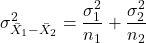
First we need to calculate the pooled variance. where v1 and v2 are degrees of freedom for sample one and sample two, respectively.
Note 1This is just simply a combined formula of the sample variance.
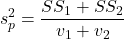
What is SS? The sum of squares , where SS1 and SS2 refer to sum of squares for each of the two groups.
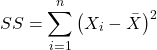
You should recognize SS from your definition of the sample variance, Chapter 3.3.
And the standard error for the difference between two means can now be written as So the 2-sample t-test can be written to reflect the pooled sample standard error of the difference between two sample means. We can see how unequal sample size is accommodated by the t-test.
Conducting the test by hand follows the same form as the one-sample t-test. Find the degrees of freedom (DF), but now for each sample.
Finally we evaluate with the critical value in Table (Appendix, Table of Student’s t distribution) and compare the t test statistic against the critical value with the appropriate degrees of freedom.
Because this is the t-test, again, we are assuming that the variances are the same between the two populations (homoscedasticity) and this allows us to pool the variance. As it turns out, the T-test is not overly sensitive to other deviations from the assumptions, but if the variances are in fact different, then the standard formula may yield incorrect Type I error rates compared to stated probability level (α).
However, it would be poor statistical choice to use a test where there are alternatives. This is why in part that R (Rcmdr) sets as the default for the t-test that variances are unequal! In fact, R does not do a t-test unless you change the default to assume equal variances, which, as we now know, is the t-test.
Welch test
What to do when assumptions to t-test are not met? Many options have been proposed, and Welch’s approximate t is a good alternative to the two-sample t-test — it would be appropriate if the normal assumption still held.
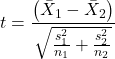
The degrees of freedom for the Welch’s test are now
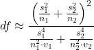
Note 2: The Welch test removes the pooled estimate of the standard error, replaces with both variance estimates directly.
As a default option, R and Rcmdr uses a variation of Welch’s test when you select to do the t-test without making the assumption of equal variance (Fig 1).
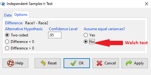
Figure 1. Screenshot Rcmdr t-test options. Default is “No” for Assume equal variances, ie, the Welch test.
The Welch test is not a nonparametric test, it is a different formulation of the t-test.
Justification for beginning with t-test
It’s unlikely that you will need the t-test in today’s research climate. Data sets are large, experiments are complex with multiple variables and samples. Why do we have to consider the t-test, and then a separate test in the case for unequal sample size? I view it as a teaching moment. It makes the general point that ALL statistical tests make assumptions about how the calculations are done and as to the nature of the data set.
This is our first experience with what to do if there is a violation of an assumption of parametric tests (see Chapter 13). Here, the assumption is that the two groups have equal sample size. When they do not, the standard t-test tends to biased estimates. On the other hand, if the assumptions are met, the standard test is the best test because it has more power to do what we intended — that is, it is best at the actual test of the null hypothesis! Take heart — this point is not always appreciated even by scientists (cf. Fagerland 2012).
Note 3: Expert advice will differ here, but you can always calculate the test statistic, even if the assumptions do not hold. The problem, the concern is with the interpretation.
Let’s us approach the problem of violation of assumptions in a couple of ways as an introduction to how, in general, to approach choice of statistical tests.
- Power of a test. Much current statistical research focuses on learning about how a particular statistical test works when assumptions are violated. Thus, in addition to learning what tests are designed to do, we need to consider the effects of violations of assumptions on the performance of the test (namely, is the Type I error at the stated alpha level?). This is a matter of statistical power; power of a test reflects how able the test is to get you the correct result even if assumptions are violated. Often tests perform well if sample sizes are large despite violation of assumptions. We mention without proving that the 2-sample T-test is robust to violations of normality assumption, to requirement for equal sample size, and even to unequal variances. But good experimental design attempts to meet the assumptions because the test does better!
- Alternate forms of some tests are available to handle some aspects of test violations. For example, the simple 2-sample T-test can be modified to accommodate different variances (Welch’s formula). Or you must find a different test (eg, nonparametric tests).
In conclusion, all tests begin with consideration of the assumptions. In some cases we can test our assumptions. For example, we learned about testing the assumption of normal distributions of sample data. We can also test the assumption of equal variances.
Questions
- Consider a clinical trial in which resting blood pressure is recorded on hypertensive subjects at the start of the trial, then 6 weeks after subjects have received daily supplements of flaxseed. Thus, for each subject there are two measures of blood pressure, BEFORE and AFTER.
- Write the null hypothesis
- Write the alternative hypothesis
- Justify why or why not the hypothesis should be two tailed. Explain why or why not an independent sample t-test may be used to compare groups.
Quiz Chapter 10.2
Digging deeper into t-test Plus the Welch test
Chapter 10 contents
- Introduction
- Compare two independent sample means
- Digging deeper into t-test Plus the Welch test
- Paired t-test
- References and suggested reading
7.6 – Confidence intervals
Quantifying uncertainty.
Although I’ve already presented the concept (eg, Chapter 3.4), and equations for confidence intervals of risk estimates (Chapter 7.4, Chapter 7.5), here, we expand on the idea of confidence intervals. Confidence intervals are a central part of meeting one of the main objectives of statistics, that is, estimation and communicating uncertainty with any reported estimate.
There are three components of statistical analysis
- Estimation
- Inference
- Modeling
Inference refers to statistical hypothesis testing — we ask questions of observations — do men (Rice et al 1999) and women (Fisher et al 2012) differ for blood glucose levels following a bout of aerobic exercise? T-tests, analysis of variance (ANOVA), chi-square, correlation, regression are types of statistical procedures used to do statistical inference. Modeling on the other hand refers to procedures used to relate cause and effect or for use in prediction of future values given new data. Many of the statistical procedures one uses for inference are also used to build statistical models (ANOVA, regression). Studies may intend to either test some hypothesis (inference) or to provide a predictive equation (modeling). But most studies that relate observations gathered from an experiment are obliged to also report statistics, and this is the realm of estimation. Estimates of the mean and standard deviation, for example, would be typical statistics one expects to find in a report. We call these descriptive statistics, and together with graphics, descriptive statistics are the chief way we describe our results.
Confidence intervals are crucial in statistics because they provide a range of values where the true population parameter is likely to fall, offering a more nuanced understanding of the estimate beyond just a single point value. Similarly, for statistical model model building, confidence intervals quantify the uncertainty inherent in data, providing a range of plausible values for model parameters rather than a single point estimate.
We will review how to calculate confidence intervals for proportions and for NNT. These intervals are available in epiR package and automatically returned in RcmdrPlugin.EBM.
Confidence interval for proportions
A proportion is the fraction of individuals in a population with some characteristic. The characteristic might be HIV positive for example. This would be called the population proportion and it would be a parameter of interest. In reality, we calculate a sample proportion and therefore estimate the population proportion with error. We can calculate the confidence interval (CI) of the proportion to communicate the precision of our estimate. For proportions, we use the binomial distribution — either a sample has the characteristic of interest or it does not — there are only two possibilities. There are a variety of ways to go here, and the simplest is to use a normal approximation. This will work well provided the sample size was reasonably large and the proportion is not close to zero or one, that is, we invoke the Central Limit Theorem here. Although the outcomes are binomial, the error is assumed to be normally distributed. The Wald confidence interval for p is

where  is the proportion of individuals with the characteristic (also called successes), z is the percentile from the normal distribution that corresponds to 1 – 1/2α. For 95% CI then α = 0.05 and z would be 1.965. (See standard normal table.) Of course, if making the normal approximation for the binomial is not appropriate, the CI is less than ideal. The binomial after all is a discrete distribution whereas the normal distribution is continuous, so errors will enter particularly for low sample numbers.
Other approaches may be used to get better estimates of CI for proportions, including Wilson score intervals and Jeffrey Intervals (Agresti and Coull 1998). See R package propCIs.
Because a statistic like the mean or a calculation of absolute or relative risk reduction are calculated from samples drawn from a population, the estimate comes with error. The error is basically this – if we calculate a statistic like number needed to treat (NNT) or its converse, the number needed to harm (NNH), we need to communicate to the reader how precise our estimate is. Estimation has to do with accuracy, error, and precision.
Confidence interval for ARR
The ARR is simply 
where  is the number of treated or exposed individuals for which the event occurred and
 is the number of untreated or unexposed individuals which the event occurred.
| Event happened | Event did not happen | |
| Treated or Exposed |
a | b |
| Control or Not exposed |
c | d |
Our data from example (Ch 7.5), were a = 612, b = 2192, c = 375, and d = 2543.

and the 95% confidence interval is then 
approximately. The “2” is only approximate; you need to use Z = 1.965, the value at probability value = 0.9725 (which comes from the Normal Table).
Confidence interval for NNT
For a sample of 100 people drawn at random from a population (which may number in the millions), then repeat the NNT calculation for a different sample of 100 people, do we expect the first and second NNT estimates to be EXACTLY the same number? No, but we do expect them to be close and we can define what we mean by close as we expect each estimate to be within certain limits. While we expect the second calculation to be close to the first estimate, we would be surprised if it was EXACTLY the same. And so, which is the correct estimate, the first or the second? They both are, in the sense that they both estimate the parameter NNT (a property of a population). But we can do better than two estimates. Confidence Intervals (CI) allow us to assign a probability to how certain we are about the statistic and whether it is likely to be close to the true value. We will
For CI of NNT, we need sample size for control and treatment groups; like all confidence intervals, we need to calculate the standard error of the statistic, in this, case, the standard error (SE) for NNT.
SE = sqrt(risk placebo * (1 - risk placebo) / (# in placebo group) + risk treatment * (1 - risk treatment) / (# in treatment group))
where SE is the standard error for NNT
The CI is approximately then 
* – the “2” is only approximate; you need to use Z = 1.965, the value at probability value = 0.9725 (by multiplying this, which comes from the Standard Normal Table).
Odds ratio Standard error and 95% confidence interval
Like any statistic we can calculate, an estimate of odds ratio should be accompanied by the confidence limit. The standard error may be calculated with the following formula

R code
seOdds <- sqrt(sum(1/612, 1/2192,1/375,1/2543))
where ln refers to the natural logarithm. An estimate for the 95% confidence interval is

where exp is the exponential function

and ln is natural logarithm.
R code
exp(log(1.89,base=exp(1)) - 1.96*seOdds)
Our example the lower limit was 1.64. For the upper limit

Our example the upper limit was 2.19.
R code
exp(log(1.89,base=exp(1)) + 1.96*seOdds)
Thus, our estimate was 1.89 and the 95% confidence interval was 
which does not include one. Therefore, we conclude statistically different.
Note 1. A reminder, log() without specifying the base returns the natural logarithm. A better coding habit might suggest always specifying the base:
log(x, base = exp(1))P-values from confidence intervals
While we expect certain reporting criteria for published, it is not uncommon that one or more elements are missing. For example, while we show how to obtain confidence intervals, the p-values were not reported. We discuss statistical inference and p-values in detail in Chapter 8, but for now, a low p-value (typically < 0.05) indicates that the odds ratio (OR) is statistically significant, meaning the observed relationship between a factor and an outcome is unlikely to be due to random chance. An OR of the difference may not be reported, or, an inexact p-value is reported like “< 0.05,” but we “need” an exact p-value for our meta-analysis. A little math, and these missing statistics can be calculated.
Note 2. We illustrated how to calculate confidence intervals from p-values in Chapter 3.4 – Estimating parameters. See two helpful “how to” articles by Bland and Altman in 2011 BMJ (references listed in Chapter 3.6 – References).
We can use the OR example. We need to take the logarithm of ratios like OR or NNT or RRR. From above, we have the confidence intervals.
We need
The OR estimate,  , which was 1.89
lower and upper confidence intervals: 1.64 and 2.19, respectively.
the standard error, which can be calculated as 
the test statistic, 
and then the p-value, 
we would then report that the OR was not statistically different, p = 0.4044).
Questions
1. Instead of 95% confidence interval, obtain the 99% confidence interval for odds ratio 1.89.
Quiz Chapter 7.6
Confidence intervals