16.2 – Causation and Partial correlation
Introduction
Science driven by statistical inference and model building is largely motivated by the the drive to identify pathways of cause and effect linking events and phenomena observed all around us. (We first defined cause and effect in Chapter 2.4) The history of philosophy, from the works of Ancient Greece, China, Middle East and so on is rich in the language of cause and effect. From these traditions we have a number of ways to think of cause and effect, but for us it will be enough to review the logical distinction among three kinds of cause-effect associations:
- Necessary cause
- Sufficient cause
- Contributory cause
Here’s how the logic works. If A is a necessary cause of B, then the mere fact that B is present implies that A must also be present. However, that the presence of A does not imply that B will occur. If A is a sufficient cause of B, then the presence of A necessarily implies the presence of B. However, another cause C may alternatively cause B. Enter the contributory or related cause: A cause may be contributory if the presumed cause A (1) occurs before the effect B, and (2) changing A also changes B. A contributory cause does not need to be necessary nor must it be sufficient; contributory causes play a role in cause and effect.
Thus, following this long tradition of thinking about causality we have the mantra, “Correlation does not imply causation.” The exact phrase was written as early as emphasized by Karl Pearson who invented the statistic back in the late 1800s. This well-worn slogan deserves to be on T-shirts and bumper stickers*, and perhaps to be viewed as the single most important concept you can take from a course in philosophy/statistics. But in practice, we will always be tempted to stray from this guidance. The developments in genome-wide-association studies, or GWAS, are designed to look for correlations, as evidenced by statistical linkage analysis, between variation at one DNA base pair and presence/absence of disease or condition in humans and animal models. These are costly studies to do and in the end, the results are just that, evidence of associations (correlations), not proof of genetic cause and effect. We are less likely to be swayed by a correlation that is weak, but what about correlations that are large, even close to one? Is not the implication of high, statistically significant correlation evidence of causation? No, necessary, but not sufficient.
Note 1. A helpful review on causation in epidemiology is available from Parascandola and Weed (2001); see also Kleinberg and Hripcsak (2011). For more on “correlation does not imply causation”, try the Wikipedia entry. Obviously, researchers who engage in genome wide association studies are aware of these issues: see for example discussion by Hu et al (2018) on causal inference and GWAS.
Causal inference (Pearl 2009; Pearl and Mackenzie 2018), in brief, employs a model to explain the association between dependent and multiple, likely interrelated candidate causal variable, which is then subject to testing — is the model stable when the predictor variables are manipulated, when additional connections are considered (eg, predictor variable 1 covaries with one or more other predictor variables in the model). Wright’s path analysis, now included as one approach to Structural Equation Modeling, is used to relate equations (models) of variation in observed variables attributed to direct and indirect effects from predictor variables.
* And yes, a quick Google search reveals lots of bumper stickers and T-shirts available with the causation  sentiment.
Spurious correlations
Correlation estimates should be viewed as hypotheses in the scientific sense of the meaning of hypotheses for putative cause-effect pairings. To drive the point home, explore the web site “Spurious Correlations” at https://www.tylervigen.com/spurious-correlations , which allows you to generate X-Y plots and estimate correlations among many different variables. Some of my favorite correlations from “Spurious Correlations” include (Table 1):
Table 1. Spurious correlations, https://www.tylervigen.com/spurious-correlations
| First variable | Second variable | Correlation |
| Divorce rate in Maine, USA | Per capita USA consumption of margarine | +0.993 |
| Honey producing bee colonies USA | Juvenile arrests for marijuana possession | -0.933 |
| Per capita USA consumption of mozzarella cheese | Civil engineering PhD awarded USA | +0.959 |
| Total number of ABA lawyers USA | Cost of red delicious apples | +0.879 |
These are some pretty strong correlations (cf. effect size discussion, Ch11.4 and 16.1), about as close to +1 as you can get. But really, do you think the amount of cheese that is consumed in the USA has anything to do with the number of PhD degrees awarded in engineering or that apple prices are largely set by the number of lawyers in the USA? Cause and effect implies there must also be some plausible mechanism, not just a strong correlation.
But that does NOT ALSO mean that a high correlation is meaningless. The primary reason a correlation cannot tell about causation is because of the problem (potentially) of an UNMEASURED variable (a confounding variable) being the real driving force (Fig 1).
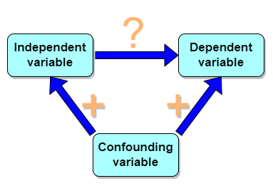
Figure 1. Unmeasured confounding variables influence association between independent and dependent variables, the characters or traits we are interested in.
Here’s a plot of running times for the best, fastest men and women runners for the 100-meter sprint. Running times over 100 meters of top athletes since the 1920s. The data are collated for you and presented at end of this page (scroll or click here).
Here’s a scatterplot (Fig 2).
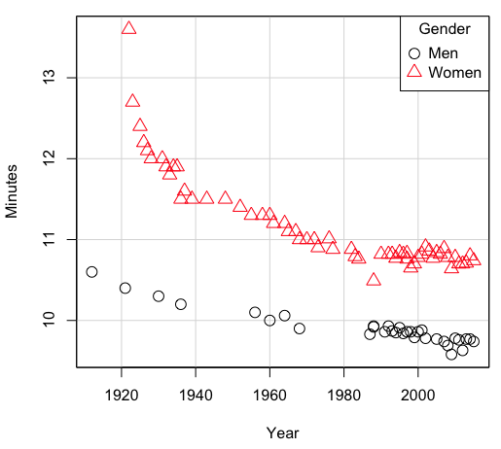
Figure 2. Running times over 100 meters of top athletes since the 1920s.
There’s clearly a negative correlation between years and running times. Is the rate of improvement in running times the same for men and women? Is the improvement linear? What, if any, are the possible confounding variables? Height? weight? Biomechanical differences? Society? Training? Genetics? … Performance enhancing drugs…?
If we measure potential confounding factors, we may be able to determine the strength of correlation between two variables that share variation with a third variable.
The partial correlation
There are several ways to work this problem. The partial correlation is a useful way to handle this problem, i.e., where a measured third variable is positively correlated with the two variable you are interested in.

Without formal mathematical proof presented, r12.3 is the correlation between variables 1 and 2 INDEPENDENT of any covariation with variable 3.
For our running data set, we have the correlation between women’s time for 100m over 9 decades, (r13 = -0.876), between men’s time for 100m over 9 decades (r23 = -0.952), and finally, the correlation we’re interested in, whether men’s and women’s times are correlated (r12 = +0.71). When we use the partial correlation, however, I get r12.3 = -0.819… much less than 0 and significantly different from zero. In other words, men’s and women’s times are not positively correlated independent of the correlation both share with the passage of time (decades)! The interpretation is that men are getting faster at a rate faster than women.
In conclusion, keep your head about you when you are doing analyses. You may not have the skills or knowledge to handle some problems (partial correlation), but you can think simply — why are two variables correlated? One causes the other to increase (or decrease) OR the two are both correlated with another variable.
Testing the partial correlation
Like our simple correlation, the partial correlation may be tested by a t-test, although modified to account for the number of pairwise correlations (Wetzels and Wagenmakers 2012). The equation for the t test statistic is now
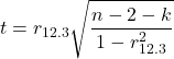
with k equal to the number of pairwise correlations and n – 2 – k degrees of freedom.
Examples
Lead exposure and low birth weigh. The data set is numbers of low birth weight births (< 2,500 g regardless of gestational age) and numbers of children with high levels of lead (10 or more micrograms of lead in a deciliter of blood) measured from their blood. Data used for 42 cities and towns of Rhode Island, United States of America (data at end of this page, scroll or click here to access the data).
A scatterplot of number of children with high lead is shown below (Fig 3).
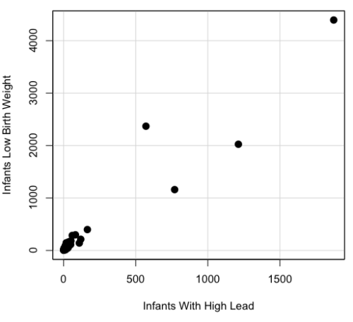
Figure 3. Scatterplot birth weight by lead exposure.
The product moment correlation was r = 0.961, t = 21.862, df = 40, p < 2.2e-16. So, at first blush looking at the scatterplot and the correlation coefficient, we conclude that there is a significant relationship between lead and low birth weight, right?
However, by the description of the data you should recall that counts were reported, not rates (eg, per 100,000 people). Clearly, population size varies among the cities and towns of Rhode Island. West Greenwich had 5085 people whereas Providence had 173,618. We should suspect that there is also a positive correlation between number of children born with low birth weight and numbers of children with high levels of lead. Indeed there are.
Correlation between Low Birth Weight and Population, r = 0.982
Correlation between High Lead levels and Population, r = 0.891
The question becomes, after removing the covariation with population size is there a linear association between high lead and low birth weight? One option is to calculate the partial correlation. To get partial correlations in Rcmdr, select
Statistics → Summaries → Correlation matrix
then select “partial” and select all three variables (select + Ctrl key; (Windows or macOS) (Fig 4).
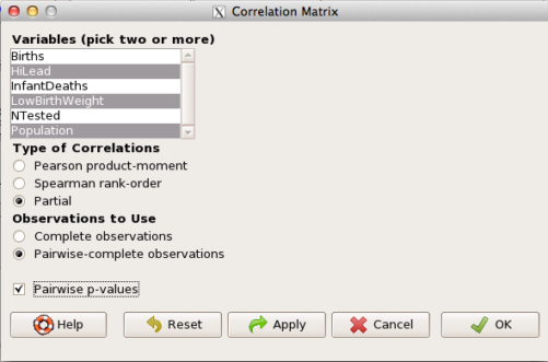
Figure 4. Screenshot Rcmdr partial correlation menu
Results are shown below.
partial.cor(leadBirthWeight[,c("HiLead","LowBirthWeight","Population")], tests=TRUE, use="complete")

Partial correlations:
                 HiLead LowBirthWeight Population
HiLead          0.00000        0.99181   -0.97804
LowBirthWeight  0.99181        0.00000    0.99616
Population     -0.97804        0.99616    0.00000
Thus, after removing the covariation we conclude there is indeed a strong correlation between lead and low birth weights.
Note 2. Some verbiage about correlation tables (matrices). The matrix is symmetric and the information is repeated. I highlighted the diagonal in green. The upper triangle (red) is identical to the lower triangle (blue). When you publish such matrices, don’t publish both the upper and lower triangles; it’s also not necessary to publish the on-diagonal numbers, which are generally not of interest. Thus, the publishable matrix would be
Partial correlations:
                LowBirthWeight Population
HiLead                 0.99181   -0.97804
LowBirthWeight                    0.99616
Another example
Do Democrats prefer cats? The question I was interested in, Do liberals really prefer cats, was inspired by a Time magazine 18 February 2014 article. I collated data on a separate but related question: Do states with more registered Democrats have more cat owners? The data set was compiled from three sources: 2010 USA Census, a 2011 Gallup poll about religious preferences, and from a data book on survey results of USA pet owners (data at end of this page, scroll or click here to access the data).
Note 3: This type of data set involves questions about groups, not individuals. We have access to aggregate statistics for groups (city, county, state, region), but not individuals. Thus, our conclusions are about groups and cannot be used to predict individual behavior, eg, knowing a person votes Green Party does not mean they necessarily share their home with a cat). See ecological fallacy.
This data set also demonstrates use of transformations of the data to improve fit of the data to statistical assumptions (normality, homoscedacity).
The variables, and their definitions, were:
ASDEMS = DEMOCRATS. Democrat advantage: the difference in registered Democrats compared to registered Republicans as a percentage; to improve the distribution qualities the arcsine transform was applied..
ASRELIG = RELIGION. Percent Religious from a Gallup poll who reported that Religion was “Very Important” to them. Also arcsine-transformed to improve normality and homoescedasticity (there you go, throwing $3 words around 🤠 ).
LGCAT = Number of pet cats, log10-transformed, estimated for USA states by survey, except Alaska and Hawaiʻi (not included in the survey by the American Veterinary Association).
LGDOG = Estimated number of pet dogs, log10-transformed for states, except Alaska and Hawaiʻi (not included in the survey by the American Veterinary Association).
LGIPC = Per capita income, log10-transformed.
LGPOP = Population size of each state, log10 transformed.
As always, begin with data exploration. All of the variables were right-skewed, so I applied data transformation functions as appropriate: log10 for the quantitative data and arc sine transform for the frequency variables. Because Democrat Advantage and Percent Religious variables were in percentages, the values were first divided by 100 to make frequencies, then the R function asin() was applied. All analyses were conducted on the transformed data, therefore conclusions apply to the transformed data.
Note 4: As we’ve discussed before, to relate the results to the original scales, back transformations would need to be run on any predictions. Back transformation for log10 would be power of ten; for the arcsine-transform the inverse of the arcsine would be used.
A scatter plot matrix (KMggplo2) plus histograms of the variables along the diagonals shows the results of the transforms and hints at the associations among the variables. A graphic like this one is called a trellis plot; a layout of smaller plots in a grid with the same (preferred) or at least similar axes. Trellis plots (Fig 5) are useful for finding the structure and patterns in complex data. Scanning across a row shows relationships between one variable with all of the others. For example, the first row Y-axis is for the ASDEMS variable; from left to right along the row we have, after the histogram, what look to be weak associations between ASDEMS and ASRELIG, LGCAT, LGDOG, and LGDOG.
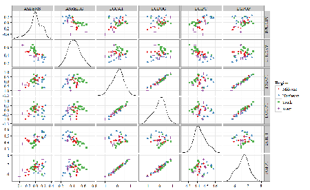
Figure 5. Trellis plot, correlations among variables.
A matrix of partial correlations was produced from the Rcmdr correlation call. Thus, to pick just one partial correlation, the association between DEMOCRATS and RELIGION (reported as “very important”) is negative (r = -0.45) and from the second matrix we retrieve the approximate P-value, unadjusted for the multiple comparisons problem, of p = 0.0024. We quickly move past this matrix to the adjusted P-values and confirm that this particular correlation is statistically significant even after correcting for multiple comparisons. Thus, there is a moderately strong negative correlation between those who reported that religion was very important to them and the difference between registered Democrats and Republicans in the 48 states. Because it is a partial correlation, we can conclude that this correlation is independent of all of the other included variables.
And what about our original question: Do Democrats prefer cats over dogs? The partial correlation after adjusting for all of the other correlated variables is small (r = 0.05) and not statistically different from zero (P-value greater than 5%).
Are there any interesting associations involving pet ownership in this data set? See if you can find it (hint: the correlation you are looking for is also in red).
Partial correlations:
         ASDEMS  ASRELIG LGCAT   LGDOG   LGIPC   LGPOP
ASDEMS   0.0000 -0.4460  0.0487  0.0605  0.1231 -0.0044
ASRELIG -0.4460  0.0000 -0.2291 -0.0132 -0.4685  0.2659
LGCAT    0.0487 -0.2291  0.0000  0.2225 -0.1451  0.6348
LGDOG    0.0605 -0.0132  0.2225  0.0000 -0.6299  0.5953
LGIPC    0.1231 -0.4685 -0.1451 -0.6299  0.0000  0.6270
LGPOP   -0.0044  0.2659  0.6348  0.5953  0.6270  0.0000
Raw P-values, Pairwise two-sided p-values:
         ASDEMS ASRELIG  LGCAT   LGDOG   LGIPC   LGPOP
ASDEMS           0.0024  0.7534  0.6965  0.4259  0.9772
ASRELIG  0.0024          0.1347  0.9325  0.0013  0.0810
LGCAT    0.7534  0.1347          0.1465  0.3473  <.0001
LGDOG    0.6965  0.9325  0.1465          <.0001  <.0001
LGIPC    0.4259  0.0013  0.3473  <.0001          <.0001
LGPOP    0.9772  0.0810  <.0001  <.0001  <.0001
Adjusted P-values, Holm’s method (Benjamini and Hochberg 1995)
         ASDEMS ASRELIG  LGCAT   LGDOG   LGIPC   LGPOP
ASDEMS           0.0241  1.0000  1.0000  1.0000  1.0000
ASRELIG  0.0241          1.0000  1.0000  0.0147  0.7293
LGCAT    1.0000  1.0000          1.0000  1.0000  <.0001
LGDOG    1.0000  1.0000  1.0000          <.0001  0.0002
LGIPC    1.0000  0.0147  1.0000  <.0001          <.0001
LGPOP    1.0000  0.7293  <.0001  0.0002  <.0001
A graph (Fig 6) to summarize the partial correlations: green lines indicate positive correlation, red lines show negative correlations; Strength of association indicated by the line thickness, with thicker lines corresponding to greater correlation.
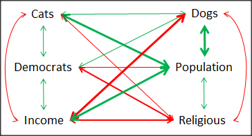
Figure 6. Causal paths among variables.
As you can see, partial correlation analysis is good for a few variables, but as the numbers increase it is difficult to make heads or tails out of the analysis. Better methods for working with these highly correlated data in what we call multivariate data analysis, for example Structural Equation Modeling or Path Analysis.
Questions
- Write up three learning outcomes for this page. Hint: Point your favorite generative AI to this page and ask for help.
- Spurious correlations can be challenging to recognize, and, sometimes, they become part of a challenge to medicine to explain away. A classic spurious correlation is the correlation between rates of MMR vaccination and autism prevalence. Here’s a table of numbers for you
| Year | Herb Supplement Revenue, millions $ | Fertility rate per 1000 births, women age 35 and older+ | MMR per 100K children age 0 -5 | UFC revenue, millions $ | Autism Prevalence per 1000 |
|---|---|---|---|---|---|
| 2000 | 4225 | 47.7 | 179 | 6.7 | |
| 2001 | 4361 | 48.6 | 183 | 4.5 | |
| 2002 | 4275 | 49.9 | 190 | 8.7 | 6.6 |
| 2003 | 4146 | 52.6 | 196 | 7.5 | |
| 2004 | 4288 | 54.5 | 199 | 14.3 | 8 |
| 2005 | 4378 | 55.5 | 197 | 48.3 | |
| 2006 | 4558 | 56.9 | 198 | 180 | 9 |
| 2007 | 4756 | 57.6 | 204 | 226 | |
| 2008 | 4800 | 56.7 | 202 | 275 | 11.3 |
| 2009 | 5037 | 56.1 | 201 | 336 | |
| 2010 | 5049 | 56.1 | 209 | 441 | 14.4 |
| 2011 | 5302 | 57.5 | 212 | 437 | |
| 2012 | 5593 | 58.7 | 216 | 446 | 14.5 |
| 2013 | 6033 | 59.7 | 220 | 516 | |
| 2014 | 6441 | 61.6 | 224 | 450 | 16.8 |
| 2015 | 6922 | 62.8 | 222 | 609 | |
| 2016 | 7452 | 64.1 | 219 | 666 | 18.5 |
| 2017 | 8085 | 63.9 | 213 | 735 | |
| 2018 | 65.3 | 220 | 800 | 25 |
- Make scatterplots of autism prevalence vs
- Herb supplement revenue
- Fertility rate
- MMR vaccination
- UFC revenue
- Calculate and test correlations between autism prevalence vs
- Herb supplement revenue
- Fertility rate
- MMR vaccination
- UFC revenue
- Interpret the correlations — is there any clear case for autism vs MMR?
- What additional information is missing from Table 2? Add that missing variable and calculate partial correlations for autism prevalence vs
- Herb supplement revenue
- Fertility rate
- MMR vaccination
- UFC revenue
- Do a little research: What are some reasons for increase in autism prevalence? What is the consensus view about MMR vaccine and risk of autism?
Quiz Chapter 16.2
Causation and Partial correlation
Data sets
Data used in this page, 100 meter running times since 1900.
| Year | Men | Women |
|---|---|---|
| 1912 | 10.6 | |
| 1913 | ||
| 1914 | ||
| 1915 | ||
| 1916 | ||
| 1917 | ||
| 1918 | ||
| 1919 | ||
| 1920 | ||
| 1921 | 10.4 | |
| 1922 | 13.6 | |
| 1923 | 12.7 | |
| 1924 | ||
| 1925 | 12.4 | |
| 1926 | 12.2 | |
| 1927 | 12.1 | |
| 1928 | 12 | |
| 1929 | ||
| 1930 | 10.3 | |
| 1931 | 12 | |
| 1932 | 11.9 | |
| 1933 | 11.8 | |
| 1934 | 11.9 | |
| 1935 | 11.9 | |
| 1936 | 10.2 | 11.5 |
| 1937 | 11.6 | |
| 1938 | ||
| 1939 | 11.5 | |
| 1940 | ||
| 1941 | ||
| 1942 | ||
| 1943 | 11.5 | |
| 1944 | ||
| 1945 | ||
| 1946 | ||
| 1947 | ||
| 1948 | 11.5 | |
| 1949 | ||
| 1950 | ||
| 1951 | ||
| 1952 | 11.4 | |
| 1953 | ||
| 1954 | ||
| 1955 | 11.3 | |
| 1956 | 10.1 | |
| 1957 | ||
| 1958 | 11.3 | |
| 1959 | ||
| 1960 | 10 | 11.3 |
| 1961 | 11.2 | |
| 1962 | ||
| 1963 | ||
| 1964 | 10.06 | 11.2 |
| 1965 | 11.1 | |
| 1966 | ||
| 1967 | 11.1 | |
| 1968 | 9.9 | 11 |
| 1969 | ||
| 1970 | 11 | |
| 1972 | 10.07 | 11 |
| 1973 | 10.15 | 10.9 |
| 1976 | 10.06 | 11.01 |
| 1977 | 9.98 | 10.88 |
| 1978 | 10.07 | 10.94 |
| 1979 | 10.01 | 10.97 |
| 1980 | 10.02 | 10.93 |
| 1981 | 10 | 10.9 |
| 1982 | 10 | 10.88 |
| 1983 | 9.93 | 10.79 |
| 1984 | 9.96 | 10.76 |
| 1987 | 9.83 | 10.86 |
| 1988 | 9.92 | 10.49 |
| 1989 | 9.94 | 10.78 |
| 1990 | 9.96 | 10.82 |
| 1991 | 9.86 | 10.79 |
| 1992 | 9.93 | 10.82 |
| 1993 | 9.87 | 10.82 |
| 1994 | 9.85 | 10.77 |
| 1995 | 9.91 | 10.84 |
| 1996 | 9.84 | 10.82 |
| 1997 | 9.86 | 10.76 |
| 1998 | 9.86 | 10.65 |
| 1999 | 9.79 | 10.7 |
| 2000 | 9.86 | 10.78 |
| 2001 | 9.88 | 10.82 |
| 2002 | 9.78 | 10.91 |
| 2003 | 9.93 | 10.86 |
| 2004 | 9.85 | 10.77 |
| 2005 | 9.77 | 10.84 |
| 2006 | 9.77 | 10.82 |
| 2007 | 9.74 | 10.89 |
| 2008 | 9.69 | 10.78 |
| 2009 | 9.58 | 10.64 |
| 2010 | 9.78 | 10.78 |
| 2011 | 9.76 | 10.7 |
| 2012 | 9.63 | 10.7 |
| 2013 | 9.77 | 10.71 |
| 2014 | 9.77 | 10.8 |
| 2015 | 9.74 | 10.74 |
| 2016 | 9.8 | 10.7 |
| 2017 | 9.82 | 10.71 |
| 2018 | 9.79 | 10.85 |
| 2019 | 9.76 | 10.71 |
| 2020 | 9.86 | 10.85 |
| 2021 | 9.77 | 10.54 |
| 2022 | 9.76 | 10.62 |
| 2023 | 9.83 | 10.65 |
| 2024 | 9.77 | 10.72 |
Data used in this page, birth weight by lead exposure
| CityTown | Core | Population | NTested | HiLead | Births | LowBirthWeight | InfantDeaths |
|---|---|---|---|---|---|---|---|
| Barrington | n | 16819 | 237 | 13 | 785 | 54 | 1 |
| Bristol | n | 22649 | 308 | 24 | 1180 | 77 | 5 |
| Burrillville | n | 15796 | 177 | 29 | 824 | 44 | 8 |
| Central Falls | y | 18928 | 416 | 109 | 1641 | 141 | 11 |
| Charlestown | n | 7859 | 93 | 7 | 408 | 22 | 1 |
| Coventry | n | 33668 | 387 | 20 | 1946 | 111 | 7 |
| Cranston | n | 79269 | 891 | 82 | 4203 | 298 | 20 |
| Cumberland | n | 31840 | 381 | 16 | 1669 | 98 | 8 |
| East Greenwich | n | 12948 | 158 | 3 | 598 | 41 | 3 |
| East Providence | n | 48688 | 583 | 51 | 2688 | 183 | 11 |
| Exeter | n | 6045 | 73 | 2 | 362 | 6 | 1 |
| Foster | n | 4274 | 55 | 1 | 208 | 9 | 0 |
| Glocester | n | 9948 | 80 | 3 | 508 | 32 | 5 |
| Hopkintown | n | 7836 | 82 | 5 | 484 | 34 | 3 |
| Jamestown | n | 5622 | 51 | 14 | 215 | 13 | 0 |
| Johnston | n | 28195 | 333 | 15 | 1582 | 102 | 6 |
| Lincoln | n | 20898 | 238 | 20 | 962 | 52 | 4 |
| Little Compton | n | 3593 | 48 | 3 | 134 | 7 | 0 |
| Middletown | n | 17334 | 204 | 12 | 1147 | 52 | 7 |
| Narragansett | n | 16361 | 173 | 10 | 728 | 42 | 3 |
| Newport | y | 26475 | 356 | 49 | 1713 | 113 | 7 |
| New Shoreham | n | 1010 | 11 | 0 | 69 | 4 | 1 |
| North Kingstown | n | 26326 | 378 | 20 | 1486 | 76 | 7 |
| North Providence | n | 32411 | 311 | 18 | 1679 | 145 | 13 |
| North Smithfield | n | 10618 | 106 | 5 | 472 | 37 | 3 |
| Pawtucket | y | 72958 | 1125 | 165 | 5086 | 398 | 36 |
| Portsmouth | n | 17149 | 206 | 9 | 940 | 41 | 6 |
| Providence | y | 173618 | 3082 | 770 | 13439 | 1160 | 128 |
| Richmond | n | 7222 | 102 | 6 | 480 | 19 | 2 |
| Scituate | n | 10324 | 133 | 6 | 508 | 39 | 2 |
| Smithfield | n | 20613 | 211 | 5 | 865 | 40 | 4 |
| South Kingstown | n | 27921 | 379 | 35 | 1330 | 72 | 10 |
| Tiverton | n | 15260 | 174 | 14 | 516 | 29 | 3 |
| Warren | n | 11360 | 134 | 17 | 604 | 42 | 1 |
| Warwick | n | 85808 | 973 | 60 | 4671 | 286 | 26 |
| Westerly | n | 22966 | 140 | 11 | 1431 | 85 | 7 |
| West Greenwich | n | 5085 | 68 | 1 | 316 | 15 | 0 |
| West Warwick | n | 29581 | 426 | 34 | 2058 | 162 | 17 |
| Woonsoket | y | 43224 | 794 | 119 | 2872 | 213 | 22 |
Data in this page, Do Democrats prefer cats?
Chapter 16 contents
- Introduction
- Product moment correlation
- Causation and Partial correlation
- Data aggregation and correlation
- Spearman and other correlations
- Instrument reliability and validity
- Similarity and Distance
- References and suggested readings
16.1 – Product moment correlation
Introduction.
A correlation is used to describe the direction  magnitude of linear association and the between two variables. There are many types of correlations, some are based on ranks, but the one most commonly used is the product-moment correlation (r). The Pearson product-moment correlation is used to describe association between continuous, ratio-scale data, where “Pearson” is in honor of Karl Pearson (b 1857 – d. 1936).
There are many other correlations, including Spearman’s and Kendall’s tau (τ) (Chapter 16.4) and ICC, the intraclass correlation (Chapter 12.3 and Chapter 16.4).
The product moment correlation is appropriate for variables of the same kind — for example, two measures of size, like the correlation between body weight and brain weight.
Spearman’s and Kendall’s tau correlation are nonparametric and would be alternatives to the product moment correlation. The intraclass correlation, or ICC, is a parametric estimate suitable for repeat measures of the same variable.
The correlation coefficient.

The numerator is the sum of products and it quantifies how the deviates from X and Y means covary together, or change together. The numerator is known as a “covariance.”

The denominator includes the standard deviations of X and Y; thus, the correlation coefficient is the standardized covariance.
The product moment correlation, r, is an estimate of the population correlation, ρ (pronounced rho), the true relationship between the two variables.
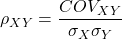
where COV(X,Y) refers to the covariance between X and Y.
Effect size.
Estimates for r range from -1 to +1; the correlation coefficient has no units. A value of 0 describes the case of no statistical correlation, ie, no linear association between the two variables. Usually, this is taken as the null hypothesis for correlation — “No correlation between two variables,” with the alternative hypothesis (2-tailed) — “There is a correlation between two variables.”
Like mean difference effect size, we can report the strength of correlation between two variables. Consider the magnitude and not the direction . Like Cohen’s effect size:
| Absolute value | Magnitude of association |
| 0.10 | small, weak |
| 0.30 | moderate |
| > 0.50 | strong, large |
Note that one should not interpret a “strong, large” correlation as evidence that the association is necessarily real. See Ch16.c for more on spurious correlations.
Standard error of the correlation.
An approximate standard error for r can be obtained using this simple formula
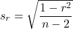
This standard error can be used for significance testing with the t-test. See below.
Confidence interval.
Like all situations in which an estimate is made, you should report the confidence interval for r. The standard error approximation is appropriate when the hull hypothesis is  , because the joint distribution is approximately normal. However, as the estimate approaches the limits of the closed interval
 , the distribution becomes increasingly skewed.
The approximate confidence interval for the correlation is based on Fisher’s z-transformation. We use this transformation to stabilize the variance over the range of possible values of the correlation and, therefore, better meet the assumptions of parametric tests based on the normal distribution.
The transform is given by the equation
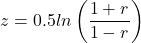
where ln is the natural logarithm. In the R language we get the natural log by log(x), where x is a variable we wish to transform.
Equivalently, z can be rewritten as

the inverse hyperbolic tangent function. In R language this function is called by atanh(r) at the R prompt.
The standard error for z is about
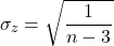
We take z to be the estimate of the population zeta, ζ. We take the sampling distribution of z to be approximately normal and thus we may then use the normal table to generate the 95% confidence interval for zeta.

Why 1.96? We want 95% confidence interval, so that at Type I α = 0.05, we want the two tails of the Normal distribution (see Appendix 20.1), or + 0.025. Thus +0.025 is +1.96 and -1.96 corresponds to 0.025 (α = 0.05/2 tails = 0.025).
Significance testing.
Significance testing of correlations is straightforward, with the noted caveat about the need to transform in cases where the estimate is close to  . For the typical test of null hypothesis, the correlation, r, is equal to 0, the t distribution can be used (ie, it’s a t-test).

which has degrees of freedom, DF = n – 2.
Use the t-table critical values to test the null hypothesis involving product moment correlation (eg, Appendix 20.3; for Spearman rank correlation  , see Table G, p. 686 in Whitlock & Schluter).
Alternatively (and preferred), we’ll just use R and Rcmdr’s facilities without explanation; the t distribution works OK as long as the correlations are not close to , in which case other things need to be done — and this is also true if you want to calculate a confidence interval for the correlation.
You are sufficiently skilled at this point to evaluate whether a correlation is statistically significantly different from zero — just check out whether the associated P-value is less than or greater than alpha (usually set at 5%). A test of whether or not the correlation, r1, is equal to some value, r2, other than zero is also possible. For an approximate test, replace zero in the above test statistic calculation with the value for r2, and calculate the standard error of the difference. Note that use of the t-test for significance testing of the correlation is an approximate test — if the correlations are small in magnitude using the Fisher’s Z transformation approach will be less biased, where the test statistic z now is

and standard error of the difference is

and look up the critical value of z from the normal table.
R code.
To calculate correlations in R and Rcmdr, have ratio-scale data ready in the columns of a R and Rcmdr data frame. We’ll introduce the commands with an example data set from my genetics laboratory course.
Question. What is the estimate of the product moment correlation between Drosophila fly wing length and area?
Data (thanks to some of my genetics students!)
Area <- c(0.446, 0.876, 0.390, 0.510, 0.736, 0.453, 0.882, 0.394, 0.503, 0.535, 0.441, 0.889, 0.391, 0.514, 0.546, 0.453, 0.882, 0.394, 0.503, 0.535)
Length <- c(1.524, 2.202, 1.520, 1.620, 1.710, 1.551, 2.228, 1.460, 1.659, 1.719, 1.534, 2.223, 1.490, 1.633, 1.704, 1.551, 2.228, 1.468, 1.659, 1.719)
Create your data frame, eg,
FlyWings <- data.frame(Area, Length)
And here’s the scatterplot (Fig 1). We can clearly see that Wing Length and Wing Area are positively correlated, with one outlier (Fig 1).
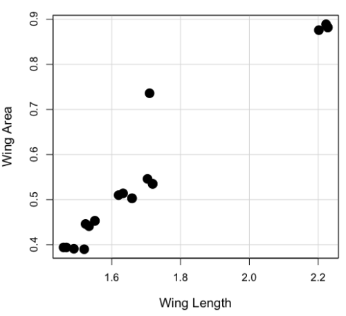
Figure 1. Scatterplot of Drosophila wing area by wing length.
The R command for correlation is simply cor(x,y). This gives the “pearson” product moment correlation, the default. To specify other correlations, use method = "kendall", or method = "spearman" (See Chapter 16.4).
Question. What are the Pearson, Spearman, and Kendall’s tau estimates for the correlation between fly Wing Length and Wing Area?
At the R prompt, type
cor(Length,Area)
[1] 0.9693334
cor(Length,Area, method="kendall")
[1] 0.8248008
cor(Length,Area, method="spearman")
[1] 0.9558658
Note that we entered Length first. On your own, confirm that the order of entry does not change the correlation estimate. To both estimate test the significance of the correlation between Wing Area and Wing Length, at the R prompt type
cor.test(Area, Length, alternative="two.sided", method="pearson")
R returns with
Pearson's product-moment correlation

data: Area and Length

t = 16.735, df = 18, p-value = 2.038e-12>
alternative hypothesis: true correlation is not equal to 0
95 percent confidence interval:
0.9225336 0.9880360
sample estimates:
   cor
0.9693334
Alternatively, to calculate and test the correlation, use R Commander, Rcmdr: Statistics → Summaries→ Correlation test
Note 1. R’s cor.test uses Fisher’s z transformation; note if we instead use the approximate calculation instead how poor the approximation works in this example. The estimated correlation was 0.97, thus the approximate standard error was 0.058. The confidence interval (t-distribution, alpha=0.05/2 and 18 degrees of freedom) was between 0.848 and 1.091, which is greater than the z transform result and returns an out-of-bounds upper limit.
Alternative packages to base R provide more flexibility and access to additional approaches to significance testing of correlations (Goertzen and Cribbie 2010). For example, z_cor_test() from the TOSTER package.
z_cor_test(Area, Length)

Pearson's product-moment correlation
data:  Area and Length
z = 8.5808, N = 20, p-value < 2.2e-16
alternative hypothesis: true correlation is not equal to 0
95 percent confidence interval:
0.9225336 0.9880360
sample estimates:
      cor
0.9693334
To confirm, check the critical value for z = 8.5808, two-tailed, with
> 2*pnorm(c(8.5808), mean=0, sd=1, lower.tail=FALSE)
[1] 9.421557e-18
Note the difference is that Fisher’s z is used for hypothesis testing; cor.test and z_cor_test return same confidence intervals.
and by bootstrap resampling (see Chapter 19.2),
boot_cor_test(Area, Length)

Bootstrapped Pearson's product-moment correlation

data: Area and Length
N = 20, p-value < 2.2e-16
alternative hypothesis: true correlation is not equal to 0
95 percent confidence interval:
0.8854133 0.9984744
sample estimates:
cor
0.9693334
The z-transform confidence interval would be preferred over the bootstrap confidence interval because it is narrower.
Assumptions of the product-moment correlation.
Interestingly enough, there are no assumptions for estimating a statistic. You can always calculate an estimate, although of course, this does not mean that you have selected the best calculation to describe the phenomenon in question, it just means that assumptions are not applicable for estimation. Whether it is the sample mean or the correlation, it is important to appreciate that, look, you can always calculate it, even if it is not appropriate!
Statistical assumptions and those technical hypotheses we evaluate apply to statistical inference — being able to correctly interpret a test of statistical significance for a correlation estimate depends on how well assumptions are met. The most important assumption for a null hypothesis test of correlation is that samples were obtained from a “bivariate normal distribution.” It is generally sufficient to just test normality of the variables one at a time (univariate normality), but the student should be aware that testing the bivariate normality assumption can be done directly (eg, Doornick and Hansen 2008).
Testing two independent correlations
Extending from a null hypothesis of the correlation is equal to zero to the correlation equals a particular value should not be a stretch for you. For example, since we use the t-test to evaluate the null hypothesis that the correlation is equal to zero, you should be able to make the connection that, like the two sample t-test, we can extend the test of correlation to any value. However, using the t-test without considering the need to stabilize the variance.
When two correlations come from independent samples, we can test whether or not the two correlations are equal. Rather than use the t-test, however, we use a modification of Fisher’s Z transformation. Calculate z for each correlation separately, then use the following equation to obtain Z. We then look up Z from our table of standard normal distribution (Appendix 20.1, or better — use the normal distribution functions in Rcmdr) and we can obtain the p-value of the test of the hypothesis that the two correlations are equal.
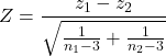
Example. Two independent correlations are r1 = 0.2 and r2 = 0.34. Sample sizes for group 1 was 14 and for group 2 was 21. Test the hypothesis that the two correlations are equal. Using R as a calculator, here’s what we might write in the R script window and the resulting output. It doesn’t matter which correlation we set as r1 or r2, so I prefer to calculate the absolute value of Z and then get the probability from the normal table for values greater or equal to |Z| (ie, the upper tail).
z1 = atanh(0.2)
z2 = atanh(0.34)
n1 = 14
n2 = 21
Z = abs((z1-z2)/sqrt((1/(n1-3))+(1/(n2-3))))
Z = 0.3954983
From the normal distribution table we get a p-value of 0.3462 for the upper tail. Because this p-value is not less than our typical Type I error rate of 0.05, we conclude that the two correlations are not in fact significantly different.
Rcmdr: Distributions → Continuous distributions → Normal distribution → Normal probabilities…
pnorm(c(0.3954983), mean=0, sd=1, lower.tail=FALSE)
R returns
[1] 0.3462376
To make this two-tailed, of course all we have to do is multiple the one-tailed p-value by two, in this case two-tailed p-value = 0.69247.
Write a function in R
There’s nothing wrong with running the calculations as written. But R allows users to write their own functions. Here’s one possible function we could write to test two independent correlations. Write the R function in the script window.
test2Corr = function(r1,r2,n1,n2) {
z1=atanh(r1); z2=atanh(r2)
Z = abs((z1-z2)/sqrt((1/(n1-3))+(1/(n2-3))))
pnorm(c(Z), mean=0, sd=1, lower.tail=FALSE)
}
After submitting the function, we then invoke the function by typing at the R prompt
p = test2Corr(0.2,0.34,14,21); p
Again, R returns the one-tailed p-value
[1] 0.3462376
Unsurprisingly, these simple functions are often available in an R package. In this case, the psych package provides a function called r.test() which will accommodate the test of the equality hypothesis of two independent correlations. Assuming that the psych package has been installed, at the R prompt we type
require(psych)
r.test(14,.2,.34,n2=21,twotailed=TRUE)
And R returns
Correlation tests
Call:r.test(n = 14, r12 = 0.20, r34 = 0.34, n2 = 21, twotailed = TRUE)
Test of difference between two independent correlations
z value 0.4 with probability 0.69
More on testing correlations
The discussion above, as stated, assumes the two correlations are independent of each other. In ecological studies, for example, it is not uncommon to have estimates for correlations among multiple pairs of traits. Thus, our approach would not be appropriate for testing whether the difference in correlations between body mass/ornament size and body mass/swimming performance of male killifish because both correlations include the same variable (body mass). A better solution would be to use William’s t-test (Williams 1959, Diedenhofen and Musch 2015).
Note 2: This example was selected from Sowersby et al 2022 — I’m not implying here that the authors analyzed their results incorrectly, I just like the example of traits to illustrate the point!
The null hypothesis was evaluated using Williams’ (1959)  -test for overlapping dependent correlations with
 degrees of freedom, calculated as:
(1) 
Where  represents the determinant of the
 correlation matrix, defined as:
(2) 
The r.test() in psyche package can be modified to handle this. R code for a made up example:
# 1. Define your sample size (N)
sample_size <- 65 # Example: 65 male killifish

# 2. Define the three correlation coefficients (r)
# r12 = correlation between body mass and ornament size
# r13 = correlation between body mass and swimming performance
# r23 = correlation between ornament size and swimming performance
r_mass_ornament <- 0.55
r_mass_swim <- 0.30
r_ornament_swim <- 0.40

# 3. Run Williams' t-test using r.test()
result <- psych::r.test(
   n = sample_size,
   r12 = r_mass_ornament,
   r13 = r_mass_swim,
  r23 = r_ornament_swim
)

# 4. View the results
print(result)
R output
Correlation tests
Call:[1] "r.test(n = 65 , r12 = 0.55 , r23 = 0.4 , r13 = 0.3 )"
Test of difference between two correlated correlations
t value 2.13 with probability < 0.037NULL
And we would conclude that the two correlations are indeed statistically different from each other.
Alternatively, use the cocor.dep.groups.overlap() from the cocor package. This generates all of the proposed tests of such correlations.
For our example then,
library(cocor)

# 1. Define sample size (N)
sample_size <- 65
# 2. Define individual correlations (r)
# r.jk = correlation between body mass (j) and ornament size (k)
# r.jh = correlation between body mass (j) and swimming performance (h)
# r.kh = correlation between ornament size (k) and swimming performance (h)
r_mass_ornament <- 0.55
r_mass_swim <- 0.30
r_ornament_swim <- 0.40
#3. Note: j is the overlapping/shared variable (body mass)
my_result <- cocor.dep.groups.overlap(
    r.jk = r_mass_ornament,
    r.jh = r_mass_swim,
   r.kh = r_ornament_swim,
   n = sample_size,
   alternative = "two.sided",
   alpha = 0.05
)

# 4. View the full comparison report
show(my_result)
Note 3: To extract and print ONLY Williams’ t-test results use my_results@williams1959.
R output (rearranged, brought William’s t-test up to the top for comparisons).
Results of a comparison of two overlapping correlations based on dependent groups

Comparison between r.jk = 0.55 and r.jh = 0.3
Difference: r.jk - r.jh = 0.25
Related correlation: r.kh = 0.4
Group size: n = 65
Null hypothesis: r.jk is equal to r.jh
Alternative hypothesis: r.jk is not equal to r.jh (two-sided)
Alpha: 0.05

williams1959: Williams' t (1959)
t = 2.1291, df = 62, p-value = 0.0372
Null hypothesis rejected

pearson1898: Pearson and Filon's z (1898)
z = 2.1217, p-value = 0.0339
Null hypothesis rejected

hotelling1940: Hotelling's t (1940)
t = 2.1635, df = 62, p-value = 0.0344
Null hypothesis rejected

olkin1967: Olkin's z (1967)
z = 2.1217, p-value = 0.0339
Null hypothesis rejected

dunn1969: Dunn and Clark's z (1969)
z = 2.0926, p-value = 0.0364
Null hypothesis rejected

hendrickson1970: Hendrickson, Stanley, and Hills' (1970) modification of Williams' t (1959)
t = 2.1635, df = 62, p-value = 0.0344
Null hypothesis rejected

steiger1980: Steiger's (1980) modification of Dunn and Clark's z (1969) using average correlations
z = 2.0795, p-value = 0.0376
Null hypothesis rejected

meng1992: Meng, Rosenthal, and Rubin's z (1992)
z = 2.0675, p-value = 0.0387
Null hypothesis rejected
95% confidence interval for r.jk - r.jh: 0.0161 0.6017
Null hypothesis rejected (Interval does not include 0)

hittner2003: Hittner, May, and Silver's (2003) modification of Dunn and Clark's z (1969) using a backtransformed average Fisher's (1921) Z procedure
z = 2.0741, p-value = 0.0381
Null hypothesis rejected

zou2007: Zou's (2007) confidence interval
95% confidence interval for r.jk - r.jh: 0.0155 0.4877
Null hypothesis rejected (Interval does not include 0)
Note 4: show() not summary() because cocor.dep.groups.overlap() returns an S4 object.
Questions
- Write up three learning outcomes for this page. Hint: Point your favorite generative AI to this page and ask for help.
- True or False. Generally, the null hypothesis of a test of a correlation is Ho: r = 0, although in practice, one could test a null of r = any value.
- Return to the fly wing example. What was the estimate of the value of the product moment correlation? The Spearman Rank correlation? The Kendall’s tau?
- OK, you have three correlation estimates for test of the same null hypothesis, ie, correlation between Length and Area is zero. Which estimate is the best estimate?
- Apply the Fisher z transformation to the estimated correlation, what did you get?
- For the fly wing example, what were the degrees of freedom?
- For the fly wing example, calculate the approximate standard error of the product moment correlation.
- Return one last time to the fly wing example. What was the value of the lower limit of the 95% confidence interval for the estimate of the product moment correlation? And the value of the upper limit?
- Assume that another group of students (n = 15) made measurements on fly wings and the correlation was 0.86. Is the difference between the two correlations for the two groups of students equal? Obtain the probability using the Z calculation and R (Chapter 6.7) or the normal table.
Quiz Chapter 16.1
Product moment correlation
Chapter 16 contents
5.3 – Replication, Bias, and Nuisance Variables
Introduction
This page describes additional elements of experimental design, replication and bias, which can impact the validity of a study.
Replication in science refers to repeating an experiment under identical conditions multiple times. To the extent the same conclusions are achieved, we can say the outcome is reproducible (Simmons 2014) and, therefore, likely to be objectively true (Earp 2011). Replication of experimental and sampling units is an essential component of good experimental design. Confusing technical replicates for biological replicates is called pseudoreplication.
Bias refers to any of a number of sociological and cognitive errors which may influence conclusions in science (Ionnidis 2005). In a meta-analysis, Fanelli et al (2017) reported that while the size of effect from identifiable biases were small, some disciplines were more prone to these sources of error. That researchers testing similar hypotheses reach different conclusions may result from bias. One such bias is positive outcome bias, where reports of null hypotheses are more often rejected than they should be based on sample size and other concerns of statistical power (see Chapter 11 – Power analysis).
The page concludes with a discussion of nuisance variables, variables that may be causally associated with the outcome of interest, but themselves are either of no interest in the study, or may not be known in advance (Meehl 1970; see also discussion of spurious correlations in Chapter 16.3 – Data aggregation and correlation).
Technical vs. biological replicates.
A laboratory technician retrieves a vial of an immortalized cell line from cryostorage and initiate propagation of the cells for the week’s work. After a couple of days of subculturing, the technician has grown millions of cells and is ready to set up an assay. After washing the cells in PBS (phosphate buffered saline), the technician adjusts the concentration of cells to 10,000 per mL media, places the tube on ice, and proceeds to set up a 48 well microplate. To each well, the technician adds media, one or more agents (Table 1), plus cells, total volume each well at one mL, three replicates per treatment.
Table 1. In our example there were four treatments plus a control (media only)
- DMSO only (D)
- DMSO + Cytokine (DC)
- DMSO + Small molecule Inhibitor (DS)
- DMSO + Cytokine + Small molecule Inhibitor (DCS)
- Media only (M)
The plate table might look something like Figure 1.

Figure 1. Schematics of a set up for a hypothetical 48 well microplate (plate_plot() from ggplate package).
The technician has done a lot of work; but, from a statistician’s point of view, effectively the technician has but one sampling unit to show for his efforts; one biological sampling unit because as far as we can tell, the cells were all related. Biological replication refers to repeat measures (eg, same conditions) on biologically distinct entities (Blainey et al 2014). Technical replication, in contrast, refers to repeat measures on the same entity, eg, the same individual (Blainey et al 2014).
However, there were more than one technical samples in the experimental design, twelve in all because there were twelve wells. Many of you will recognize this as the distinction between technical and biological replicates. In thinking about experimental design replicates pertain to the number of sampling units that are treated the same way. In our example cells may be “treated the same way” in at least two distinct ways. Biologically, the cells may be the same: derived from the same clonal cell, all at the same passage (generation) number, each cell genetically, morphologically, physiologically (etc.,) identical to the next cell. Technical replication on the other hand pertains to the levels of the treatments.
Within each of these treatments we had three wells, and that’s at the level of the technical replication.
A final note on this experiment. We as molecular biologists call each of these treatment groups, but statisticians thinking of this design would recognize only one treatment (called in statistics a factor), with four levels of the treatment. We will discuss this beginning in chapter 12 when we introduce analysis of variance.
Types of bias.
When we make decisions, we like to think we are rational; that we make decisions based on an evaluation of evidence. And yet, an increasing body of literature suggests that our decisions often made in a manner that falls short of rational processing. We outlined some sources of bias in Chapter 2.6. Deviance from rational decision making is due to any number of cognitive biases we may have. Researchers and medical doctors make many decisions and, unfortunately, are just as susceptible to cognitive biases as the rest of us. One kind of bias that is bedeviling to research is confirmatory bias. Confirmatory bias refers to a researcher in effect seeking evidence in a way that confirms a prior conclusion (Kaptchuck 2003). Confirmatory bias would be exhibited if we report positive effects of aspirin to relieve migraines in subjects, but exclude cases where the subjects report no improvement. Medical doctors may be risk averse and therefore tend to over-prescribe, or they may be risk-takers (eg, rise and fall of high-dose chemotherapy, cf, discussion in Howard et al. 2011).
The concept of bias was first introduced in Chapter 3 and will be returned to in subsequent chapters. In general, bias refers to the objectivity of measurement and inferences about such measurements. Bias implies that a series of measurements consistently fail to return the true value of the variable. Bias is systematic error and may be associated with a poorly calibrated instrument or even the use of improper sets of rules for measurement given the nature of the characteristic. Bias can be captured by the concept of accuracy.
Bias is challenging to eliminate; the best way is to design the experiment so that the observer, the researcher, is unaware of the specific questions to be tested. The research is conducted “blind.” Clinical research provides the easiest examples. A trial can be blind in a couple of ways:
- The subjects do not know which treatment they receive, but the researcher does know
- The researcher does not know which treatment subjects receive, but the subjects know
- Neither the researcher nor the subjects know which treatment they receive.
- The other possibility is that both the researcher and the subjects know treatments received — this would be a poor design.
Bias can enter a research project at multiple levels. A partial list of sources of bias in research includes (modified after Pannucci and Wikins 2010):
Bias that occurs before the experiment
- Inadequate planning of the experiment, flawed design
- Bias in selection of subjects from the reference population
- Surveillance bias, where one group is studied more closely than another group.
Surveillance bias, also called detection bias or ascertainment bias, a type of information bias. Characterized as “the more you look, the more you find (Sackett 1979),” differences in outcome counts varies with differences in effort to detect. Recently, cases of myocarditis in young people were reported following Covid-19 mRNA vaccination (eg, Bozkurt et al 2021. Marshall et al 2021). However, myocarditis reports following vaccination occur at the rates expected in the population, and the reports lack important context (eg, other respiratory viruses known to cause myocarditis not ruled out), suggesting the putative link between Covid-19 vaccines and this heart condition may be result of us looking hard for signs of adverse effects of the vaccine (cf, discussion in O’Leary and Maldonado 2021).
Bias during the experiment
- Interviewer bias
- Chronology bias
- Recall bias
- Transfer bias
- Misclassification of exposure or outcome
- Performance bias
Performance bias refers to conditions of an experiment that introduce unintended differences between groups. For example, subjects enrolled in a weight-loss study randomly assigned to the control group may react poorly when they realize they are not receiving the experimental intervention. This leads to potential for a systematic bias — participants in the control group may behave differently, counteracting the point of randomization (McCambridge et al 2014).
Another well-known performance bias is associated with eliciting maximal performance from animals, such as running stamina or maximum sprint running speed (Losos et al 2002). For example, spring running speed of lizards may be measured by placing lizards onto a high-speed treadmill, then increasing belt speed to match the individual’s burst performance (eg, Dohm et al 1998). Clearly, not all individuals will perform to maximum physiological capabilities under these conditions.
Bias after the experiment
- Citation bias
- Confounding
Another way to view sources of bias is that, at least from the perspective of the researcher, the bias is likely to be unconscious bias. After all, if we knew about the sources of bias we would work our experiments in such a way to minimize known error producing sources (Holman et al 2015). Selecting subjects at random and keeping record keeping blind with respect to treatments are among the best tools we have to avoid this kind of bias.
Nuisance variables
A key quality of experimental design is the opportunity afforded the researcher to apply control. In a classic view of the experiment, one allows only one aspect to vary, the treatment applied, all else is controlled. Thus, any difference in outcome may be attributed to the treatment. However, it is likely impossible to control for all possible variables that may affect our outcome; confounding clear interpretation of results (see Chapter 16.2 and 16.3). Consider, for example, the effects of age on running performance (Fig. 2).
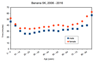
Figure 2. Mean 5K running times (minutes) by age and gender (2006 – 2016, Jamba Juice Banana 5K race, Honolulu, HI).
If we are interested in gender differences, we must also deal with the change in performance with age: older runners regardless of gender tend to run slower than younger runners. Thus, in the comparison of genders, age is a nuisance variable. In the literature, you may see “lurking variable,” or other such names. The concept is that these variables may be causal, but are either of no interest in the study, or may not be known in advance. Therefore, age must be accounted for before we can address gender differences, if any. Age, in this case, is considered a nuisance variable because we are not primarily interested in age effects, but age clearly covaries (is associated) with running performance. How best to handle nuisance variables? One approach is to match by age (blocking effect, see Chapter 14.4); another approach would be to randomly select with respect to age when compiling female and male times.
Another example of confounding. Results from ecological experiments intended to test for presence of competition for resources by plant species by removing plants may alter herbivory levels; thus, survivorship not the result of reduced plant-plant competition but because of changes in herbivore behavior (Reader 1992).
Questions
- I cite a number of articles in Mike’s Biostatistics Book. If you’re paying attention, you’ll have noticed that all of my citations, at least for articles, link to a source that you can either download or read online. What kind of error am I committing by following this approach?
- In large part because of the tendency for overuse of antibiotics, doctors are less likely today to prescribe antibiotics for patients with upper respiratory tract infections than in the past (Zoorob et al 2012). URTI are mostly caused by rhinovirus infections (Calderaro et al 2022) and, therefore, the course of infection in a patient should be unaffected by addition of antibiotic. However, although rare compared to URTI, life-threatening illness like acute epiglottitis caused by bacteria infection can sometimes develop or accompany URTI. Thus, not prescribing antibiotics at a diagnosis of URTI may risk a worsening condition for the patients. This sets the doctor up for a potential cognitive bias – to prescribe or not to prescribe antibiotics prophylactically? Discuss this decision in the context of potential sources of cognitive biases and possible outcomes of the decision.
Quiz Chapter 5.3
Replication, bias, and nuisance variables
Chapter 5 contents
- The basics explained
- Experiments
- Experimental and Sampling units
- Replication, Bias, and Nuisance Variables
- Clinical trials
- Importance of randomization in experimental design
- Sampling from Populations
- References and suggested readings