5.6 – Sampling from Populations
Introduction
Researchers generally can’t study an entire population. More generally, striving to study each member of a population is not necessary to arrive at answers about the population. For example, consider the question, does taking a multivitamin daily improve health? What are our options? Do we really need to follow every single individual in the United States of America, monitoring their health and noting whether or not the person takes vitamins daily in order to test (inference) this hypothesis? Or, can we get at the same answer by careful experimental design (see Schatzkin et al 2002; Dawsey et al 2014)? Supplement use is wide-spread in the United States, but both health and vitamin use differ by demographics. Young people tend to be healthier than older people and older people tend to take supplements more than younger people.
A subset of the population is measured for some trait or characteristic. From the sample, we hope to refer back to the population. We want to move from anecdote (case histories) to possible generalizations of use to the reference population (all patients with these symptoms). How we sample from the reference population limits our ability to generalize. We need a representative sample: simple to define, hard to achieve.
Statistics becomes necessary if we want to infer something about the entire populations. (Which is usually the point of doing a study!!) Typically tens to thousands of individuals are measured. But in addition, HOW we obtain the sample of individuals from the reference population is CRITICAL.
Kinds of sampling include (adapted from Box 1, Tyrer and Heyman 2016; see also McGarvey et al 2016)
Probability sampling
- random
- stratified
- blocking
- clustered
- systematic
Nonprobability sampling
- convenience, haphazard
- judgement
- quota
- snowball
For an exhaustive, authoritative look at sampling, see Thompson (2012).
How can samples be obtained?
Sampling from a population may be convenient. For one famous example, consider the Bumpus data set. (We introduced this data set in Question 5, Chapter 5.) So the legend goes, Professor Bumpus was walking across the campus of Brown University, the day after a severe winter storm, and came across a number of motionless house sparrows on the ground. Bumpus collected the birds and brought them to his lab. Seventy-two birds recovered; 64 did not (Table1).
Table 1. A subset of Bumpus data set, summarized by sex of birds.
| House sparrows | Lived | Died |
|---|---|---|
| Female | 21 | 28 |
| Male | 51 | 36 |
Bumpus reported differences in body size that correlated with survival (Bumpus 1899), and this report is often taken as an example of Natural Selection (cf. Johnston et al 1972). The Bumpus dataset is clearly convenience sampling. It’s also a case study: a report of a single incident. But given that is is a large sample (n = 136), it is tempting to use the data to inform about about possible characteristics of the birds that survived compared with those that perished.
Another way we collect samples from populations is best termed haphazard. In graduate school I got the opportunity to study locomotor performance of whiptail lizards (Aspidoscelis tigris, A. marmoratus, genus formerly Cnemidophorus**) across a hybrid zone in the Southwest United States (Dohm et al. 1998). During the day we would walk in areas where the lizards were known to occur and capture any individual we saw by hand. (This would sometimes mean sticking our hands down into burrows, which was always exciting — you never really knew if you were going to find your lizard or if you were going to find a scorpion, venomous spider, or …) Lizards collected were returned to the lab for subsequent measures. Clearly, this was not convenience sampling; it involved a lot of work under the hot sun. But just as clearly, we could only catch what we could see and even the best of us would occasionally lose a lizard that had been spotted. Moreover, one suspects we missed many lizards that were present, but not in our view. Lizards that were underground at the time we visited a spot would not be seen nor captured by us; individual lizards that were especially wary of people (Bulova 1994) would also escape us. In other words, we caught the lizards that were catchable and can only assume (hope?) that they were representative of all of these lizards. Applying a grid or quadrant system to the area and then randomly visiting plots within the grid or quadrant might help, but still would not eliminate the potential for biased sampling we faced in this study.
Quota sampling implies selection of subjects by some specific criteria, weighted by the proportions represented in the population. It’s different from stratified sampling because there is no random selection scheme: subjects are selected based on matching some criteria, and collection for that group stops when the sample number matches the proportion in the population. Consider our vitamin supplement survey. If student population at Chaminade University was the reference population, and we have enough money to survey 100 students, then we would want a sample of 70 women students and 30 male students, representing the proportions of the student population.
Snowball sampling implies that you rely on word-of-mouth to complete sampling. After initial recruitment of subjects, sample size for the study increases because early participants refer others to the researchers. This can be a powerful tool for reaching underrepresented communities (eg, Valerio et al 2016).
Types of Probability sampling
Random sampling is an example of probability sampling. As we defined earlier, simple random sampling requires that you know how many subjects are in the population (N) and then each subject has an equal chance of being selected

Examples of nonprobability sampling include
- convenience sampling
- volunteer sampling
- judgement sampling
Convenience sampling (the first 20 people you meet at the library lanai); volunteer sampling (you stand in front of a room of strangers and ask for any ten people to come forward and take your survey — or more seriously, persons with a terminal disease calling a clinic reportedly known to cure the disease with a radical new, experimental treatment), and judgement sampling (to study tastes in fashion, you decide that only persons over six feet tall should be included because .…).
Random in statistics has a very important, strict meaning. As opposed to our day-to-day usage, random sampling from a population means that the probability that any one individual is chosen to be included in a sample is equal. Formally, this is called simple random sampling to distinguish it from more complex schemes. For a sampling procedure to be random requires a formal procedure for sampling a population with known size (N).
For example, at the end of the semester, I may select the order for student presentations at random. Thus, students in the classroom would be considered the population (groups of students are my sample unit, not individual students!). What is the probability that your group will be called first? Second? We need to know how many groups there are to conduct simple random sampling. Let’s take an extreme and say that all groups have a size of one; there are 26 students in this room, so

or

of being selected first.
Now to determine the probability of your group being selected second, we need to distinguish between two kinds of sampling:
- Sampling with replacement — after I select the first group, the first group is returned to the pool of groups that have not been selected. In other words, with replacement, your group could be selected first and selected second! The probability of being selected second then remains

.
- Sampling without replacement — after I select the first group, then I have

groups left to select the second group, so probability that your group will be second is

. The first group has already been selected and is not available.
Random sampling refers to how subjects are selected from the target, reference population. Random assignment, however, describes the process by which subjects are assigned to treatment groups of an experiment. Random sampling applies to the external validity of the experiment: to the extent that a truly random sample was drawn, then results may be generalized to the study population. Random assignment of subjects to treatment however makes the experiment internally valid: results from the experiment may be interpreted in terms of causality.
R code, sample without replacement
sample(26)
[1] 1 10 11 23 17 13 8 6 19 20 21 16 14 15 5 2 12 4 26 22 9 7 25 18 3 24
R code, sample with replacement
mySample <- sample(26, replace = TRUE); mySample
[1] 9 26 24 9 3 1 23 14 26 6 5 19 17 23 11 12 3 8 7 19 2 16 3 11 1 1
How many elements duplicated?
out <- duplicated(mySample); table(out)
out
FALSE TRUE
17 9
More on sampling in R discussed in Sampling with computers below.
Additional sampling schemes
Simple random sampling is not the only option, but in many cases it is the most desirable. Consider our multivitamin study again. Perhaps studying the entire USA population is a bit extreme. How about working from a list of AARP members, sending out questionnaires to millions of persons on this list, getting back about 20% of the questionnaires, sorting through the responses and identifying the respondent to diet categories and multivitamin use. The researchers had nearly 500,000 persons willing and able to participate in their prospective study (Schatzkin et al 2001; Dawsey et al 2014; Lim et al 2021). It’s an enormous study. But is this really much better than our described lizard experiment? Let’s count the ways: Not all older people are members of AARP (that 500,000? That’s less than 1% of the 50 and older persons in the USA); A large majority of AARP members did not return surveys; Some fraction of the returned surveys were not usable; How representative of diverse aged populations in the United States is AARP?
Simple random sampling may not be practical, particularly if sub-populations, or strata, are present and members of the different sub-populations are not available to the researcher in the same numbers. In ecology, habitat-use studies routinely need to account for the patchiness of the environment in space and time (Wiens 1976; Summerville and Crisp 2021). Thus, samples are drawn in such a way to represent the frequency within each sub-population.
For a simple example, researchers conducting a controlled breeding program of mice don’t use simple random sampling to choose pairs of mates; after all, random sampling without regard of sex of the mice would lead to some pairings of males only, or females only (Fig 1).
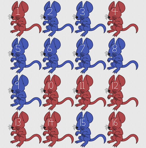
Figure 1. Sixteen mice, eight red and eight blue. Image © 2024 Mia D Graphics
R code
pairs <- c(rep("red", 8), rep("blue", 8))
replicate(2, sample(pairs, 8), simplify = FALSE)
[[1]]
[1] "blue" "blue" "blue" "red" "blue" "red" "blue" "red"

[[2]]
[1] "blue" "blue" "red" "red" "red" "red" "red" "blue"
Oops. If we interpret the output blue = male and red = female, then four out of the eight pairs were same sex pairings.
Thus, the breeding strategy is to random sample from female mice and from male mice and the stratification is sex of the mouse. Alternatively, breeders may select mice to form breeding pairs systematically: From a large colony with dozens of cages, the breeder may select one mouse from every third cage.
Stratified Random Sampling: Individuals in the population are classified into strata or sub-groups: age, economic class, ethnicity, gender, sex …, as many as needed. Then choose a simple random sample from each group, typically in proportion to the size of the sub-groups in the population. Combine those into the overall sample. For example, when I wanted a random sample of mice for my work, I called the supplier and requested that a total of 100 male and female mice be randomly selected from the five colonies they maintained. The reference population is the entire supply of mice at that company (at that time), but I wished to make sure that I got unrelated mice, so I needed to divide the population into groups (the five colonies) before my sample was constructed.
Note 1: The size of the population must be known in advance, just like in simplified random sampling. A more interesting example, the Social Security Administration conducts surveys of popular baby names by year. They post the top ten most popular names based on 1% or 5% (first strata), then by male/female (second strata).
For a simple example of the need for stratified sampling, consider our 16 blue and red mice again. If mice were randomly assigned to treatment group, then by chance unequal samples within strata may be assigned to a treatment group, potentially biasing our conclusions (Fig 2).
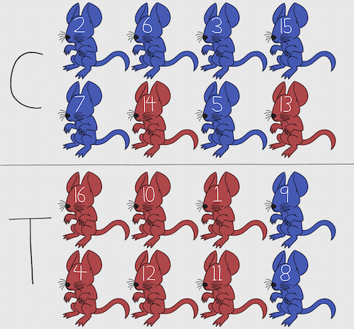
Figure 2. Sixteen mice, randomly assigned to treatment groups C and T; by chance, 75% blue in C and just 25% in T. If color was a confounding factor then our conclusions about the effectiveness of the treatment would be associated with color. Image © 2024 Mia D Graphics
Block sampling: superficially resembles stratified sampling, but refers to how experimental units are assigned to treatment groups. Blocks in experimental design refers to potentially confounding factors for which we wish to control, but are otherwise not interested in. For our example described in Figure 2, mouse color may not be of specific interest for our study and therefore would be considered a blocking effect.
Agricultural research provides a host of other blocking situations: plots distributed across an elevation or hydration gradient (Fig 3), soil types, and many others.

Figure 3. Agricultural fields in Central Poland. NASA https://visibleearth.nasa.gov/images/146593/agriculture-fields-in-central-poland/146595w
For a microbiology example, edge effects of heated culture plates. For a growth experiment it’s unlikely we are specifically interested in the plate layout on the growth characteristics of treated cells. However, it’s also unlikely we can assume placement has no influence on growth (eg, Mansoury et al 2021). A 96-well microplate has 60 inner wells and 36 edge wells (A1 – H1, A12-H12, plus 1st and 12th wells of columns B – H, for a total of 36 wells, Fig 4). Thus, analysis of growth effects should include a block effect for well position.
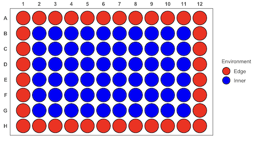
Figure 4. Format of 96-well plate. Red cells = “edge” wells; blue cells = “inner” wells. Plotted with ggplate package.
For long incubation periods it’s not unexpected that edge wells and inner wells may evaporate at different rates, potentially confounding interpretation of treatment effects if, by chance, treatment samples are more commonly assigned to edge wells. Block sampling implies subjects from treatment groups are randomly assigned to each block, in equal numbers if possible.
Cluster Sampling: In many situations, the population is far too large or too dispersed and scattered for a list of the entire population to be known. And, a random approach ignores that there is a natural grouping — people live next to each other, so there is going to be things in common. A multi-stage approach to sampling will be better than simply taking a random sample approach. Most surveys of opinion (when conducted reputably) use a multi-stage method. For example, if a senator wishes to poll his constituents about an issue, he may his pollster will randomly select a few of the counties from his state (first stage), then randomly select among towns or cities (second stage), to obtain a list of 1000 people to call. In some instances, they might use even more stages. At each stage, they might do a stratified random sample on sex, race, income level, or any other useful variable on which they could get information before sampling. If you are interested in this kind of work, for starters, see Couper and Miller (2009).
There are more types of sampling, and entire books written about the best way to conduct sampling. One important thing to keep in mind is that as long as the sample is large relative to the size of the population, each of the above methods generally will get the same answers (= the statistics generated from the samples will be representative of the population).
As long as some attempt is made to randomize, then you can say that the procedure is probability sampling. Nonprobability, or haphazard sampling, describes the other possibility, that is, each element is selected arbitrarily by a non-formal selecting of individual. … all the fish or birds that you catch may not be a random sample of those present in a population. For example,
- wild Pacific salmon do not feed on the surface, hatchery salmon feed on the surface. …
- all the individuals who respond to a survey.
- Phone surveys, web surveys, person on the street surveys… how random, how representative?
Sampling with computers
Now to determine the probability of your group being selected second, we need to distinguish between two kinds of sampling:
Sampling with replacement — after I select the first group, the first group is returned to the pool of groups that have not been selected. In other words, with replacement, your group could be selected first and selected second! The probability of being selected second then remains
Sampling without replacement — after I select the first group, then I have

groups left to select the second group, so probability that your group will be second is

. The first group has already been selected and is not available, and so on.
Sampling is usually easiest if a computer is used. Computers use algorithms to generate pseudo-random numbers. We call the resulting numbers pseudo-random to distinguish them from truly random physical processes (eg, radioactive decay). For more information about random numbers, please see random.org.
If all you wish to do is select a few observations or you need to use a random procedure to select subjects prior to observations, then these websites can provide a very quick, useful tool.
Sampling in Microsoft Excel or LibreOffice Calc
Microsoft’s Excel is pretty good at sampling, but requires knowledge of included functions. Here are the steps to generate random numbers and select with and without replacement in Excel. I’ll give you two cases.
1. For random numbers, enter the function =rand() in a cell, then drag the cell handle to fill in cells to N (in our case = 26, so A1 to A26). This function generates a random (more or less!) number between 0 and 1. We want digits between 1 and 26, not fractions between 0 and 1, so combine INT function with RAND function
=INT(27*RAND())
Note 2: To get between 1 and 9, multiply by 10 instead of 27; to get between 1 and 100, multiply by 101, etc.
In Excel to sample with replacement, simply pick the first two cells (the algorithm Excel used already has conducted sample with replacement. See next item for method to sample without replacement in Excel. You have to have installed the Data Analysis Tool Pak. Here’s instructions for Office 2010.
If you have a Mac and Office 2008, there is no Data Analysis Tool Pak, so to get this function in your Excel, install a third-party add-in program (eg, StatPlus, a free add-in, really nice, adds a lot of function to your Excel). If you have the 2011 version of Office for Mac, then the Data Analysis Tool Pak is included, but like your Windows counterparts, you have to install it (click here for instructions).
2. Let’s say that we have already given each group a number between 1 and 26 and we enter those numbers in sequence in column A.
To sample without replacement, select Tools → Data Analysis… (if this option is not available, you’ll have to add it — see Excel help for instructions, Fig 5).
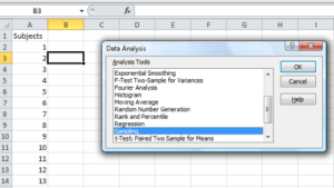
Figure 5. Screenshot of Sampling in Data Analysis menu, Microsoft Excel
Enter the cells with the numbers you wish to select from. In our example, column A has the numbers 1 through 26 representing each group in our class. I entered A:A as the Input Range.
Next, select “Random” and enter the number of samples. I want two.
Click OK and the output will be placed into cell B3 (my choice); I could have just as easily had Excel put the answer into a new worksheet.
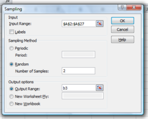
Figure 6. Screenshot of input required for Sampling in Data Analysis menu, Microsoft Excel
To sample with replacement from column A (with our 1 through 26), type in the formula B1
=INT(27*RAND())and the formula C1
=INDEX(A:A,RANK(B1,B:B))then drag the cell handles to fill in the columns (first column B, then column C).
That’ll do it for MS Excel or LibreOffice Calc.
Sampling with R (Rcmdr)
It’s much easier with much more control to get sampling in Rcmdr (R) than in Excel. Sampling in R is based on the function called sample() and sample.int(). I will present just the sample() command here.
sample(x, size, replace = FALSE, prob = NULL)Example
You want to sample ten integers between 1 and 10
sample(10)R output
sample(10)
[1]  5  1 10  8  7  3  4  9  2  6
You have a list of subjects, A1 through A10
subjects = c("A1","A2","A3","A4","A5","A6","A7","A8","A9","A10")
sample(subjects, 3, replace = FALSE, prob = NULL)
R output
sample(subjects, 3, replace = FALSE, prob = NULL)
[1] "A5" "A2" "A9"
Could use this to arrange random order for ten subjects
sample(subjects, 10, replace = FALSE, prob = NULL)
[1] "A9" "A3" "A8" "A2" "A1" "A4" "A10" "A7" "A5" "A6"
Try with replacement; To sample with replacement, type in TRUE after replace in the sample() function. The R output follows
sample(x, 10, replace = TRUE, prob = NULL)
[1]  5  5  3  5  3  7  3  5 10  6
R’s randomness is based on pseudonumbers and is, therefore, not truly random (actually, this is true of just about all computer-based algorithms unless they are based on some chaotic process). We can use this pseudo part to our advantage: if we want to reproduce our “random” process, we can seed the random number algorithm to a value (eg, 100), with the command in the Script Window
set.seed(100)For 10 random integers (eg, observations), type in the Script window
sample(10)R returns the following in the Output Window
sample(10)
[1] 4 5 7 3 10 9 2 1 6 8
Sampling was done without replacement. Here’s another selection round,
First without setting a seed value
sample(10)
[1] 10 4 7 3 8 1 2 9 6 5
Try again to see if get the same 10
sample(10)
[1]  1  4  8  2  9  6  5 10  3  7
Now to demonstrate how setting the seed allows you to draw repeated samples that are the same.
Note 3: If I need to precede the sample command with a set.seed() call, then sampling is repeatable.
set.seed(100)
sample(10)
[1] 4 3 5 1 9 6 10 2 8 7
and try again
set.seed(100)
sample(10)
[1] 4 3 5 1 9 6 10 2 8 7
Additional R packages that help with sampling schemes include: sampling() and spatialsample, which is part of the BiodiversityR package, which is available as a plugin for R Commander.
Quiz Chapter 5.6
Sampling from populations
Questions
- For our two descriptions of experiments in section 6.1 (the sample of patients; the sample of frogs), which sampling technique was used?
- What purpose is served by
set.seed()in a sampling trial? - Consider our question, Does taking a multivitamin daily improve health? Imagine you have a grant willing to support a long-term prospective study to follow up to one thousand people for ten years. List at least three concerns with proposed solutions about how sampling of subjects for the study.
- Imagine you wish to conduct a detailed survey to learn about student preferences. Your survey will include many questions, so you decide to ask just ten students. Student population is 70% female, 30% male.
- Assuming you select at random (simple random sampling), what is the chance that no male students will be included in your survey?
- You are able to increase the number of surveys to 20, 30, 40, or 50. What is the chance that no male students will be included in your survey for each of these increased sample numbers?
- What can you conclude about the effects of increasing survey sample size on representativeness of students for the survey?
- Discuss how you could apply a stratified sampling scheme to this survey and whether or not this approach improves representativeness.
- Why are random numbers generated by a computer called pseudo random numbers?
Chapter 5 contents
5.5 – Importance of randomization in experimental design
Introduction
If the goal of the research is to make general, evidenced-based statements about causes of disease or other conditions of concern to the researcher, then how the subjects are selected for study directly impacts our ability to make generalizable conclusions. The most important concept to learn about inference in statistical science is that your sample of subjects upon which all measurements and treatments are conducted, ideally should be a random selection of individuals from a well-defined reference population.
The primary benefit of random sampling is that it strengthens our confidence in the links between cause and effect. Often after an intervention trial is complete, differences among the treatment groups will be observed. Groups of subjects who participated in sixteen weeks of “vigorous” aerobic exercise training show reduced systolic blood pressure compared to those subjects who engaged in light exercise for the same period of time (Cox et al 1996). But how do we know that exercise training caused the difference in blood pressure between the two treatment groups? Couldn’t the differences be explained by chance differences in the subjects? Age, body mass index (BMI), overall health, family history, etc?
How can we account for these additional differences among the subjects? If you are thinking like an experimental biologist, then the word “control” is likely coming to the foreground. Why not design a study in which all 60 subjects are the same age, the same BMI, the same general health, the same family … history…? Hmm. That does not work. Even if you decide to control age, BMI, and general health categories, you can imagine the increased effort and cost to the project in trying to recruit subjects based on such narrow criteria. So, control per se is not the general answer.
If done properly, random sampling makes these alternative explanations less likely. Random sampling implies that other factors that may causally contribute to differences in the measured outcome, but themselves are not measured or included as a focus of the research study, should be the same, on average, among our different treatment groups. The practical benefits of proper random sampling is that recruiting subjects gets easier — fewer subjects will be needed because you are not trying to control dozens of factors that may (or may not!) contribute to differences in your outcome variable. The downside to random sampling is that the variability of the outcomes within your treatment groups will tends to increase. As we will see when we get to statistical inference, large variability within groups will make it less likely that any statistical difference between the treatment groups will be observed.
Demonstrate the benefits of random sampling as a method to control for extraneous factors.
The study reported by Cox et al included 60 obese men between the ages of 20 and 50. A reasonable experimental design decision would suggest that the 60 subjects be split into the two treatment groups such that both groups had 30 subjects for a balanced design. Subjects who met all of the research criteria and who had signed the informed consent agreement are to be placed into the treatment groups and there are many ways that group assignment could be accomplished. One possibility, the researchers could assign the first 30 people that came into the lab to the Vigorous exercise group and the remaining 30 then would be assigned to the Light exercise group. Intuitively I think we would all agree that this is a suspect way to design an experiment, but more importantly, why shouldn’t you use this convenient method?
Just for argument’s sake, imagine that their subjects came in one at a time, and, coincidentally, they did so by age. The first person was age 21, the second was 22, and so on up to the 30th person who was 50. Then, the next group came in, again, coincidentally in order of ascending age. If you calculate the simple average age for each group you will find that they are identical (35.5 years). On the surface, this looks like we have controlled for age: both treatment groups have subjects that are the same age. A second option is to sort the subjects into the two treatment groups so that a 21 year old is in Group A, and the other 21 year old is in Group B, and so on. Again, the average age of Group A subjects and of Group B subjects would be the same and therefore controlled with respect to any covariation between age and change in blood pressure. However, there are other variables that may covary with blood pressure, and by controlling one, we would need to control the others. Randomization provides a better way.
I will demonstrate how randomization tends to distribute the values in such a way that the groups will not differ appreciably for the nuisance variables like age and BMI differences and, by extension, any other covariable. The R work is attached following the Reading list. The take-home message: After randomly selecting subjects for assignment to the treatment groups, the apparent differences between Group A and Group B for both age and BMI are substantially diminished. No attempt to match by age and by BMI is necessary. The numbers are shown in the table and then in two graphics (Fig 1, Fig 2) derived from the table.
Table 1. Mean age and BMI for subjects in two treatment groups A and B where subjects were assigned randomly or by convenience to treatment groups.
| Group | Random assignment of subjects to treatment groups | Convenience assignment of subjects to treatment groups |
|---|---|---|
| A | 35.2 | 28 |
| B | 35.8 | 43 |
| A | 32.49 | 28.99 |
| B | 32.87 | 37.37 |
Just for emphasis, the means from Table 1 are presented in the next two figures (Fig 1 and Fig 2).
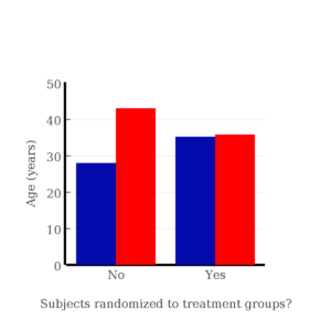
Figure 1. Age of subjects by groups (A = blue, B = red) with and without randomized assignment of subjects to treatment groups.
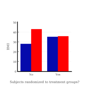
Figure 2. BMI of subjects by groups (A = blue, B = red) with and without randomized assignment of subjects to treatment groups.
Note that the apparent difference between A and B for BMI disappear once proper randomization of subjects was accomplished. In conclusion, a random sample is an approach to experimental design that helps to reduce the influence other factors may have on the outcome variable (eg, change in blood pressure after 16 weeks of exercise). In principle, randomization should protect a project because, on average, these influences will be represented randomly for the two groups of individuals. This reasoning extends to unmeasured and unknown causal factors as well.
This discussion was illustrated by random assignment of subjects to treatment groups. The same logic applies to how to select subjects from a population. If the sampling is large enough, then a random sample of subjects will tend to be representative of the variability of the outcome variable for the population and representative also of the additional and unmeasured cofactors that may contribute to the variability of the outcome variable.
What about observational studies? How does randomization work?
However, if you do cannot obtain a random sample, then conclusions reached may be sample-specific, biased. …perhaps the group of individuals that likes to exercise on treadmills just happens to have a higher cardiac output because they are larger than the individuals that like to exercise on bicycles. This nonrandom sample, an example of confounding where an extraneous or nuisance variable, body size, is associated with both the independent variable (exercise preference) and the dependent variable (cardiac output), will bias your results and can lead to incorrect interpretation of results.
Alternatively, perhaps a researcher elects to study the cardiac output of treadmill users versus bicycle users. The researcher sets up their testing station inside a gym’s powerlifting zone, where the largest individuals in the gym hang out. Inevitably because of this choice, the researcher over recruits larger individuals into the treadmill group, leading to a falsely elevated average cardiac output for treadmill users. This is an example of ascertainment bias — the sample is not representative of all treadmill users at the gym.
Random sampling is CRUCIAL in epidemiology, opinion survey work, most aspects of health, drug studies, medical work with human subjects. It’s difficult and very costly to do… so most surveys you hear about, especially polls reported from Internet sites, are NOT conducted using random sampling (included in the catch-all term “probability sampling“)!! As an aside, most opinion survey work involves complex sample designs involving some form of geographic clustering (eg, all phone numbers in a city, random sample among neighborhoods).
Random sampling is the ideal if generalizations are to be made about data, but strictly random sampling is not appropriate for all kinds of studies. Consider the question of whether or not EMF exposure is a risk factor for developing cancer (Pool 1990). These kinds of studies are observational: at least in principle, we wouldn’t expect that housing and therefore exposure to EMF is manipulated (cf. discussion Walker 2009). Thus, epidemiologists will look for patterns: if EMF exposure is linked to cancer, then more cases of cancer should occur near EMF sources compared to areas distant from EMF sources. Thus, the hypothesis is that an association between EMF exposure and cancer occurs non-randomly, whereas cancers occurring in people not exposed to EMF are random. Unfortunately, clusters can occur even if the process that generates the data is random.
Compare Graph A and Graph B (Fig 3). One of the graphs resulted from a random process and the other was generated by a non-random process. Note that the claim can be rephrased about the probability that each grid has a point, eg, it’s like Heads/Tails of 16 tosses of a coin. We can see clusters of points in Graph B; Graph A lacks obvious clusters of points — there is a point in each of the 16 cells of the grid. Although both patterns could be random, the correct answer in this case is Graph B.
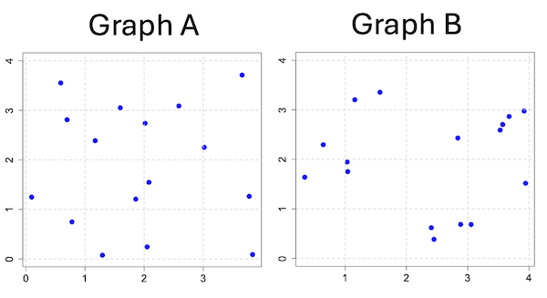
Figure 3. An example of clustering resulting from a random sampling process (Graph B). In contrast, Graph A was generated so that a point was located within each grid.
Hard to tell — and truth be told, random process could generate either one. To convince you, Figure 4 reveals the grouping that was done for Group A, in contrast with Group B which was drawn with the truly random process.
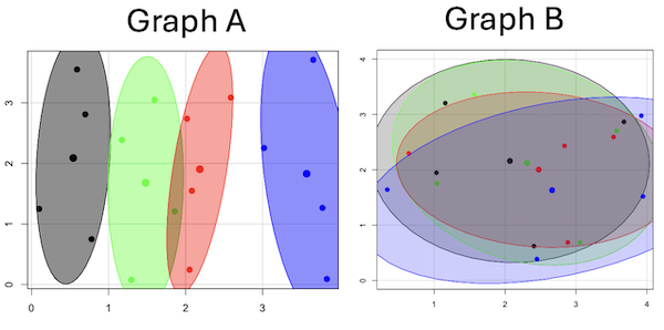
Figure 4. Same graphs as Figure 3, but with ellipses around the grouped data (hard to tell, but the centroids are the larger points).
Implications for sampling
The graphic below shows the transmission grid in the continental United States (Fig 5). How would one design a random sampling scheme overlaid against the obviously heterogeneous distribution of the grid itself? If a random sample was drawn, chances are good that no population would be near a grid in many of the western states, but in contrast, the likelihood would increase in the eastern portion of the United States where the population and therefore transmission grid is more densely placed.
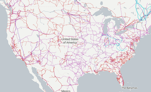
Figure 5. Map of electrical transmission grid for continental United States of America. Image source https://openinframap.org/#3/24.61/-101.16
For example, you want to test whether or not EMF affects human health, and your particular interest is in whether or not there exists a relationship between living close to high voltage towers or transfer stations and brain cancer. How does one design a study, keeping in mind the importance of randomization for our ability to generalize and assign causation? This is a part of epidemiology which strives to detect whether clusters of disease are related to some environmental source. It is an extremely difficult challenge. For the record, no clear link to EMF and cancer has been found, but reports do appear from time to time (eg, report on a cluster of breast cancer in men working in office adjacent to high EMF, Milham 2004).
Questions
1. Use the sample() with and without replacement on the object (see help with R below)
fruit <- c("apple", "banana", "grape", "kiwi", "pear", "pineapple", "tomato")a) set of 3
b) set of 4
2. Confirm the claim by calculating the probability of Graph A result vs Graph B result (see R script below).
Quiz Chapter 5.5
Importance of randomization in experimental design
R code!
Code you type is shown in red; responses or output from R are shown in blue. Recall that statements preceded by the hash # are comments and are not read by R (ie, no need for you to type them).
First, create some variables. Vectors aa and bb contain my two age sequences.
 aa = seq(21,50)
 bb = seq(21,50)
Second, append vector bb to the end of vector aa
 age = append(aa,bb)
 age           #submit the vector (variable) name to print the records for verification - looks good!
  [1] 21 22 23 24 25 26 27 28 29 30 31 32 33 34 35 36 37 38 39 40 41 42 43 44 45 46 47 48 49 50 21 22 23 24 25 26 27 28 29 30 31 32 33 34 35 36 37
 [48] 38 39 40 41 42 43 44 45 46 47 48 49 50
Third, get the average age for the first group (the aa sequence) and for the second group (the bb sequence). Lots of ways to do this, I made a two subsets from the combined age variable; could have just as easily taken the mean of aa and the mean of bb (same thing!).
 A = age[1:30]
 mean(A)
 [1] 35.5
 B = age[31:60]
 mean(B)
 [1] 35.5
Fourth, start building a data frame, then sort it by age. Will be adding additional variables to this data frame
 ex.random = data.frame(age)
 AO.all = sort(ex.random$age)
 AO.age           #submit the vector (variable) name to print the records for verification - looks good!
  [1] 21 21 22 22 23 23 24 24 25 25 26 26 27 27 28 28 29 29 30 30 31 31 32 32 33 33 34 34 35 35 36 36 37 37 38 38 39 39 40 40 41 41 42 42 43 43 44
 [48] 44 45 45 46 46 47 47 48 48 49 49 50 50
Fifth, divide the variable again into two subsets of 30 and get the averages
 AO = AO.age[1:30]
 AO
  [1] 21 21 22 22 23 23 24 24 25 25 26 26 27 27 28 28 29 29 30 30 31 31 32 32 33 33 34 34 35 35
 mean(AO)
 [1] 28
 BO = AO.age[31:60]
 BO
  [1] 36 36 37 37 38 38 39 39 40 40 41 41 42 42 43 43 44 44 45 45 46 46 47 47 48 48 49 49 50 50
 mean(BO)
 [1] 43
Sixth, create an index variable, random order without replacement
rand.index = sample(1:60,60,replace=F)Add the new variable to our existing data frame, then print it to check that all is well
 ex.random$rand = rand.index
 ex.random
    age rand
 1   21   43
 2   22   15
 3   23   17
 4   24   35
 5   25   19
 6   26   18
 7   27   22
 8   28   31
 9   29   12
 10  30   44
 11  31   24
 12  32    5
 13  33    2
 14  34   50
 15  35   23
 16  36   20
 17  37   41
 18  38   56
 19  39   36
 20  40    8
 21  41   45
 22  42   38
 23  43   42
 24  44   46
 25  45   16
 26  46   21
 27  47   28
 28  48   10
 29  49   32
 30  50   54
 31  21   57
 32  22   51
 33  23   27
 34  24   40
 35  25   14
 36  26   48
 37  27   26
 38  28   58
 39  29    9
 40  30   11
 41  31    4
 42  32   52
 43  33   37
 44  34   53
 45  35    6
 46  36   34
 47  37   39
 48  38    7
 49  39    1
 50  40   47
 51  41   33
 52  42   60
 53  43   49
 54  44   30
 55  45   29
 56  46   55
 57  47   13
 58  48    3
 59  49   25
 60  50   59
Seventh, select for our first treatment group the first 30 subjects from the randomized index. There are again other ways to do this, but sorting on the index variable means that the subject order will be change too.
AR.age = ex.random[order(ex.random$rand),] #created a new data frame to distinguish it from the presorted version "ex.random"Print the new data frame to confirm that the sorting worked. It did. we can see that the rows have been sorted by ascending order based on the index variable.
 AR.age
    age rand
 49  39    1
 13  33    2
 58  48    3
 41  31    4
 12  32    5
 45  35    6
 48  38    7
 20  40    8
 39  29    9
 28  48   10
 40  30   11
 9   29   12
 57  47   13
 35  25   14
 2   22   15
 25  45   16
 3   23   17
 6   26   18
 5   25   19
 16  36   20
 26  46   21
 7   27   22
 15  35   23
 11  31   24
 59  49   25
 37  27   26
 33  23   27
 27  47   28
 55  45   29
 54  44   30
 8   28   31
 29  49   32
 51  41   33
 46  36   34
 4   24   35
 19  39   36
 43  33   37
 22  42   38
 47  37   39
 34  24   40
 17  37   41
 23  43   42
 1   21   43
 10  30   44
 21  41   45
 24  44   46
 50  40   47
 36  26   48
 53  43   49
 14  34   50
 32  22   51
 42  32   52
 44  34   53
 30  50   54
 56  46   55
 18  38   56
 31  21   57
 38  28   58
 60  50   59
 52  42   60
Eighth, create our new treatment groups, again of n = 30 each, then get the means ages for each group.
 AR = AR.age$age[1:30]
 mean(AR)
 [1] 35.16667
 AR2 = AR.all$all[31:60]
 mean(AR2)
 [1] 35.83333
Get the minimum and maximum values for the groups
 min(AR)
 [1] 22
 min(AR2)
 [1] 21
 max(AR)
 [1] 49
 max(AR2)
 [1] 50
Ninth, create a BMI variable drawn from a normal distribution with coefficient of variation equal to 20%. The first group with we will call cc
cc = rnorm(n=30,m=27.5, sd=5.5) #mean was 27.5 for this group with standard deviation of 5.5The second group called dd
dd = rnorm(n=30,m=37.5, sd=7.5) #mean was 37.5 for this group with standard deviation of 7.5Create a new variable called BMI by joining cc and dd
 BMI=append(cc,dd)
 BMI            #print out BMI to confirm. Looks good!
  [1] 27.87528 27.83250 31.88703 34.99041 24.06751 23.50952 22.57779 31.48394 31.04321 25.60258 25.41081 22.34619 34.62213 36.41348 41.17740
 [16] 20.56529 27.25238 21.85205 32.11690 32.37168 23.11314 33.29110 34.99106 38.22016 18.72105 26.22030 25.13412 27.50475 34.79361 32.81267
 [31] 47.57872 27.58428 40.17211 38.22195 26.91893 37.02784 53.72671 34.94727 30.35245 38.32571 40.52111 36.15627 30.36592 36.20397 47.63142
 [46] 40.30846 36.47643 50.86804 43.63741 37.84994 42.82665 41.71008 28.44976 24.57906 42.37762 38.38512 35.22879 31.34063 34.02996 27.28038
Add the BMI variable to our data frame.
 ex.random$BMI = BMI
 ex.random              #Print out the revised data frame. Looks good. We now have three variables: age, the index "rand," and now BMI
    age rand      BMI
 1   21   43 27.87528
 2   22   15 27.83250
 3   23   17 31.88703
 4   24   35 34.99041
 5   25   19 24.06751
 6   26   18 23.50952
 7   27   22 22.57779
 8   28   31 31.48394
 9   29   12 31.04321
 10  30   44 25.60258
 11  31   24 25.41081
 12  32    5 22.34619
 13  33    2 34.62213
 14  34   50 36.41348
 15  35   23 41.17740
 16  36   20 20.56529
 17  37   41 27.25238
 18  38   56 21.85205
 19  39   36 32.11690
 20  40    8 32.37168
 21  41   45 23.11314
 22  42   38 33.29110
 23  43   42 34.99106
 24  44   46 38.22016
 25  45   16 18.72105
 26  46   21 26.22030
 27  47   28 25.13412
 28  48   10 27.50475
 29  49   32 34.79361
 30  50   54 32.81267
 31  21   57 47.57872
 32  22   51 27.58428
 33  23   27 40.17211
 34  24   40 38.22195
 35  25   14 26.91893
 36  26   48 37.02784
 37  27   26 53.72671
 38  28   58 34.94727
 39  29    9 30.35245
 40  30   11 38.32571
 41  31    4 40.52111
 42  32   52 36.15627
 43  33   37 30.36592
 44  34   53 36.20397
 45  35    6 47.63142
 46  36   34 40.30846
 47  37   39 36.47643
 48  38    7 50.86804
 49  39    1 43.63741
 50  40   47 37.84994
 51  41   33 42.82665
 52  42   60 41.71008
 53  43   49 28.44976
 54  44   30 24.57906
 55  45   29 42.37762
 56  46   55 38.38512
 57  47   13 35.22879
 58  48    3 31.34063
 59  49   25 34.02996
 60  50   59 27.28038
Tenth, repeat our protocol from before: Set up two groups each with 30 subjects, calculate the means for the variables and then sort by the random index and get the new group means.
 AO = ex.random$BMI[1:30]
 mean(AO)
 [1] 28.99333
 BO = ex.random$BMI[31:60]
 mean(BO)
 [1] 37.36943
All we did was confirm that the unsorted groups had mean BMI of around 27.5 and 37.5 respectively. Now, proceed to sort by the random index variable. Go ahead and create a new data frame
 AR.age = ex.random[order(ex.random$rand),]
 AR.age                 #Print out the new data frame to confirm. Looks good.
    age rand      BMI
 49  39    1 43.63741
 13  33    2 34.62213
 58  48    3 31.34063
 41  31    4 40.52111
 12  32    5 22.34619
 45  35    6 47.63142
 48  38    7 50.86804
 20  40    8 32.37168
 39  29    9 30.35245
 28  48   10 27.50475
 40  30   11 38.32571
 9   29   12 31.04321
 57  47   13 35.22879
 35  25   14 26.91893
 2   22   15 27.83250
 25  45   16 18.72105
 3   23   17 31.88703
 6   26   18 23.50952
 5   25   19 24.06751
 16  36   20 20.56529
 26  46   21 26.22030
 7   27   22 22.57779
 15  35   23 41.17740
 11  31   24 25.41081
 59  49   25 34.02996
 37  27   26 53.72671
 33  23   27 40.17211
 27  47   28 25.13412
 55  45   29 42.37762
 54  44   30 24.57906
 8   28   31 31.48394
 29  49   32 34.79361
 51  41   33 42.82665
 46  36   34 40.30846
 4   24   35 34.99041
 19  39   36 32.11690
 43  33   37 30.36592
 22  42   38 33.29110
 47  37   39 36.47643
 34  24   40 38.22195
 17  37   41 27.25238
 23  43   42 34.99106
 1   21   43 27.87528
 10  30   44 25.60258
 21  41   45 23.11314
 24  44   46 38.22016
 50  40   47 37.84994
 36  26   48 37.02784
 53  43   49 28.44976
 14  34   50 36.41348
 32  22   51 27.58428
 42  32   52 36.15627
 44  34   53 36.20397
 30  50   54 32.81267
 56  46   55 38.38512
 18  38   56 21.85205
 31  21   57 47.57872
 38  28   58 34.94727
 60  50   59 27.28038
 52  42   60 41.71008
Get the means of the new groups
 AR = AR.age$BMI[1:30]
 mean(AR)
 [1] 32.49004
 min(AR)
 [1] 18.72105
 max(AR)
 [1] 53.72671
 AR2 = AR.all$BMI[31:60]
 mean(AR2)
 [1] 33.87273
 min(AR2)
 [1] 21.85205
 max(AR2)
 [1] 47.57872
That’s all of the work!
Data set
nonrandom
| X | Y |
| 0.779 | 0.747 |
| 0.098 | 1.248 |
| 0.697 | 2.811 |
| 0.59 | 3.553 |
| 1.295 | 0.075 |
| 1.858 | 1.207 |
| 1.172 | 2.388 |
| 1.597 | 3.051 |
| 2.051 | 0.242 |
| 2.081 | 1.546 |
| 2.016 | 2.738 |
| 2.587 | 3.088 |
| 3.833 | 0.088 |
| 3.776 | 1.264 |
| 3.017 | 2.254 |
| 3.657 | 3.712 |
random
| X1 | Y1 |
| 1.157 | 3.203 |
| 2.407 | 0.62 |
| 1.033 | 1.946 |
| 3.676 | 2.866 |
| 3.57 | 2.703 |
| 3.056 | 0.685 |
| 1.568 | 3.355 |
| 1.041 | 1.753 |
| 0.643 | 2.295 |
| 2.884 | 0.687 |
| 3.53 | 2.591 |
| 2.838 | 2.431 |
| 3.945 | 1.518 |
| 0.34 | 1.64 |
| 2.45 | 0.386 |
| 3.921 | 2.976 |
Chapter 5 contents
- The basics explained
- Experiments
- Experimental and Sampling units
- Replication, Bias, and Nuisance Variables
- Clinical trials
- Importance of randomization in experimental design
- Sampling from Populations
- References and suggested readings