6.7 – Normal distribution and the normal deviate (Z)

Introduction

In chapter 3.3 we introduced the normal distribution and the Z score, aka normal deviate, as part of a discussion about how some knowledge about characteristics of the dispersion of our data sampled from a population could be used to calculate how many samples we need (the empirical rule). We introduced Chebyshev’s inequality as a general approach to this problem, where little is known about the distribution of the population and contrasted it with the Z score, for cases where the distribution is known to be Gaussian or the normal distribution. The normal distribution is one of the most important distributions in classical statistics. All normal distributions are bell-shaped and symmetric about the mean. To describe a normal distribution only two parameters are needed: the population mean, μ, and the population standard deviation, σ. The normal distribution with mean equal to zero and standard deviation equal to one is called the standard normal, or Z distribution. With use of the Z score any normal distribution can be quickly converted to the standard normal distribution.

Proportions of a Normal Distribution

This concept will become increasingly important for the many statistical tests we will learn over the next few weeks. What is the proportion of the populations that is greater than some specific value? Below (Fig 1), again, I have generated a large data set, now with population mean µ = 5 and σ = 2. The red line corresponds to the equation of the normal curve using our values of µ = 5 and σ = 2.

Figure 1. Frequency of observations expected to be greater than 7 (red bars) from a large population with mean µ = 5 and σ = 2.

R code for Fig 1.

set.seed(123)
myData <- rnorm(1000, mean = 5, sd = 2)
h <- hist(myData, breaks = 20, plot = FALSE) 
threshold <- 7
# Bars with midpoints greater than threshold will be "red", 
# and others will be "white."
bar_colors <- ifelse(h$mids > threshold, "red", "white")
plot(h, col = bar_colors, xlab = "Value", ylab = "Frequency")

Note that this is a crucial step! We assume that our sample distribution is really a sample from a population density (= “area under the curve”) function (= “an equation”) for a normal random (= “population”) variable.

Once I (you) make this assumption, then we have powerful and easy to use tools at our command to answer questions like

Question: What proportion of the population is greater than 7 (Fig 1, colored in red)?

This gets to the heart of the often-asked question, How many samples should I measure? If we know something about the mean and the variability, then we can predict how many samples will be of a particular kind. Let’s solve the problem.

The Z score

We could use the formula for the normal curve (and a lot of repetitions), but fortunately, some folks have provided tables that short-cut this procedure. R and other programs also can find these numbers because the formulas are “built in” to the base packages. First, let’s introduce a simple formula that lets us standardize our population numbers so that we can use established tables of probabilities for the normal distribution.

Below, we will see how to use Rcmdr for these kinds of problems.

However, it’s one of the basic tasks in statistics that you should be able to do by hand. We’ll use the Z score as a way to take advantage of known properties of the standard normal curve.

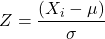
Z = 1 (with the mean and SD). Z (say “Z-score”) is called the normal deviate (aka “standard normal score”; it is also called the “Z-score”); it gives us a shortcut for finding the proportion of data greater than 7 in this case).

We use the normal deviate to do a couple of things; one use is to standardize a sample of observations so that they have a mean of zero and a standard deviation of one (the Z distribution). The data would then said to have been normalized.

The second use is to make predictions about how often a particular observation is likely to be encountered. As you can imagine, this last use is very helpful for designing an experiment — if we need to see a specified difference, we can conduct a pilot study (or refer to the literature) to determine a mean and level of variability for our observation of choice, plug these back into the normal equation and predict how likely we can expect to see a particular difference. In other words, this is one way to answer that question — how many observations need I make for my experiment to be valid?

Table of normal distribution

A portion of the table of the normal curve is provided at our web site and in your workbook. For our discussions, here’s another copy to look at (Fig 2).

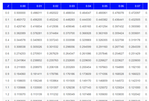
Figure 2. Portion of the table of the normal distribution. Only values equal to or greater than Z = 0 are visible.

See Table 1 in the Appendix for a full version of the normal table.

We read values of Z from the first column and the first row. For Z = 0.23 we would scan the top row, scoot over to fourth column, then trace to where the row and column intersect (Fig 3); the frequency of occurrence of values at Z = 0.23 is 0.409046 or 40.9% (Fig 3).

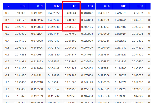
Figure 3. Highlight Z = 0.23, frequency is 0.409046.

Z on the standard normal table is going to range between -4 and +4, with Z = 0 corresponding to 0.500. The Normal table values are symmetrical about the mean of zero.

What to make of the values of Z, from -4, -3, … +2, +3, up to +4 and beyond?  These are the standard deviations! Recall that using the Z score you corrected to mean of zero (got it!), and a standard deviation of one! A Z of 2 is twice the standard deviation; a Z = 3 is therefore three times the standard deviation, and so forth. The distribution is symmetrical: you get the same frequency for negative as for positive values. So on the “X” axis on a standard normal distribution, we have units of standard deviation plus (greater) or minus (less) than the mean. In Figure 4, area less than -1 standard deviations is highlighted (Fig 4).

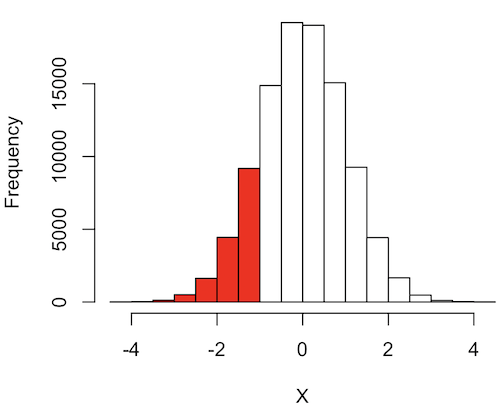
Figure 4. Plot of standard normal distribution; area less than -1 σ.

R code for Fig 4.

set.seed(123)
myData2 <- rnorm(100000, mean = 0, sd = 1)
threshold <- -1
bar_colors <- ifelse(h$mids < threshold, "red", "white")
# Additional code used, same as Figure 1.

Question. How many multiples of standard deviations would you have for a Z score of Z = 1.75?

Answer = 1.75 times

Examples

See Table 1 in the Appendix for a full version of the normal table as you read this section.

What proportion of the data set will have values greater than 7? After applying our Z score equation, I get Z = 1.0 and for a Z of 1.0 = 0.1587 or 15.87% of the observations are greater than 7.

What proportion of the data set will have values less than -7? After applying our Z score equation, I get Z = -1.0. Taking advantage of symmetry argument, I just take my Z = -1.0 and make it positive — instead of values smaller than -1.0 we now have values greater than +1.0. And for a Z of 1.0 = 0.1587 or 15.87% of the observations are greater than 7, which means that 15.87% will be -7 or smaller.

What proportion of the data set will have values greater than 8? Again, apply the Z score equation I get Z of 1.5 = 0.0668 or 6.68% of the observations are greater than Z.

What proportion of the population is between 5 and 7 ? (colored in red). Draw the problem (example shown in Fig 5).

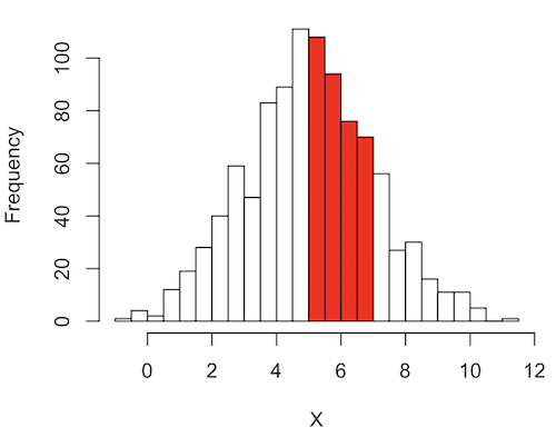
Figure 5. Proportion of the population is between 5 and 7.

R code for Fig 5.

# Used myData from Fig 1 code.

highlight_start <- 5
highlight_end <- 7
bar_colors <- rep("white", length(h$counts)) 
bar_colors[h$breaks[-length(h$breaks)] >= highlight_start & h$breaks[-1] <= highlight_end] <- "red"
# Additional code used, same as Figure 1.

Worked problem

1 – (proportion beyond 7) – (proportion less than 5)

1 – (0.1587) – (proportion less than 5)

And the proportion less than 5?

Use Z-score equation again. Now we find that

Z = 0

And look up Z of 0 from the table  = 0.5 proportion or 50.0%

Therefore, the proportion between 5 & 7 equals

1 -0.1587 – 0.50 = 0.3413

Answer = 34.13 % of the observations are between 5 and 7 when the mean µ = 5 and s = 2.

Questions

Several questions were asked in the text.

1. Proportion of observations greater than 7  from a large population with mean µ = 5 and σ = 2.

2. How many multiples of standard deviations would you have for a Z score of Z = 1.75?

3.

Quiz Chapter 6.7

Normal distribution questions

Start Quiz

Question

✕

✓

Your answer:

Correct answer:

Next

Please wait..

↺

You got {{SCORE_CORRECT}} out of {{SCORE_TOTAL}}

Your Answers

Chapter 6 contents

• Introduction
• Some preliminaries
• Ratios and probabilities
• Combinations and permutations
• Types of probability
• Discrete probability distributions
• Continuous distributions
• Normal distribution and the normal deviate (Z)
• Moments
• Chi-square (Χ²) distribution
• t distribution
• F distribution
• References and suggested readings

6.6 – Continuous distributions

Large numbers and the Central Limit Theorem

Imagine we’ve collected (sampled) data from a population and now want to summarize the data sample. How do we proceed? A good starting point is to plot the data in a histogram and note the shape of the sample distribution. Not to get too far ahead of ourselves here, but much of the classical inferential statistics demands that we are able to assume that the sampled values come from a certain kind of distribution called the normal, or Gaussian distribution.

Consider a random sample drawn from a normally distributed population of the following series of graphs, Figures 1 – 4:

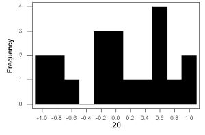
Figure 1. Sample size = 20, drawn from population with known μ = 0 and σ = 1.

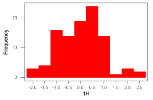
Figure 2. Sample size = 100, also drawn from population with known μ = 0 and σ = 1.

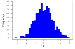
Figure 3. Sample size n = 1000, once again drawn from population with known μ = 0 and σ = 1.

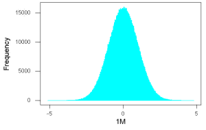
Figure 4. And lastly, sample size n = 1 million also drawn from population with known μ = 0 and σ = 1.

These graphs illustrate a fundamental point in statistics: for many kinds of measurements in biology, the more data you sample, the more likely the data will approach a normal distribution. This series of simulations was a quick and dirty “proof” of the Central Limit Theorem, which is one of the two fundamental theorems of probability, the other being that of Law of Large Numbers (ie, large-sample statistics). Basically the CLT says that for a large number of random samples, the sample mean will approach the population mean,  μ, and the sample variance will approach the population variance σ²; the distribution of the large sample will converge on the normal distribution.

As the sample size gets bigger and bigger, the resulting sample means and standard deviations get closer and closer to the true value (remember — I TOLD the program to grab numbers from the Z distribution with a mean of zero and standard deviation = 1), obeying the Law of Large Numbers.

Simulation

I used the computer to generate sample data from a population. This process is called a simulation. R can make new data sets by sampling from known populations with specified distribution properties that we determine in advance — a very powerful tool — a technique used for many kinds of statistics (eg, Monte Carlo methods, bootstrapping, etc., see Chapter 19).

1. The first graph is for a sample of 20 points;
2. the second for 100;
3. the third for 1,000;
4. and lastly, 1 million points.

To generate a sample from a normal population, the Rcmdr call the menu by selecting:

Rcmdr: Distributions → Continuous distributions → Normal distribution → Sample from normal distribution…

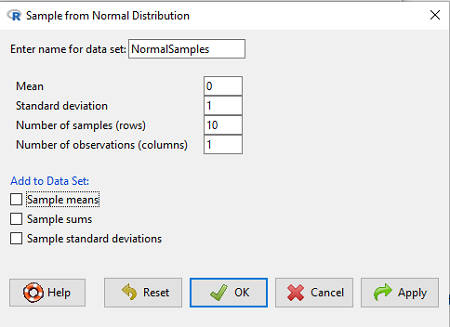
Figure 5. Screenshot Rcmdr menu, sample from a normal distribution.

The menu pops up. I entered Mean (μ) = 0 and Standard deviation (σ) = 1 number of samples = 10, unchecked all boxes under the “add to data set.” I left the object name as “NormalSamples,” you can, of course, change it as needed. R code derived from these requests were

normalityTest(~obs, test="shapiro.test", data=NormalSamples)
NormalSamples <- as.data.frame(matrix(rnorm(10*1, mean=0, sd=1), ncol=1))
rownames(NormalSamples) <- paste("sample", 1:10, sep="")
colnames(NormalSamples) <- "obs"

This results in a new data.frame called NormalSamples with a single variable called obs.

for (i in 1:3){
print(rnorm(5))
}
[1] -0.4221672 -1.4317800 -1.8310352 0.4181184 -1.1596058
[1] -0.2034944 1.1809083 1.5925296 -2.0763677 1.6982357
[1] -1.0967218 -0.3205041 -1.7513838 -0.3335311 -1.8808454

for (i in 1:3){
set.seed(1) 
print(rnorm(5))
}
[1] -0.6264538 0.1836433 -0.8356286 1.5952808 0.3295078
[1] -0.6264538 0.1836433 -0.8356286 1.5952808 0.3295078
[1] -0.6264538 0.1836433 -0.8356286 1.5952808 0.3295078

After creating a sample of numbers drawn from the normal distribution, make a histogram, Rcmdr: Graphs → Histogram… (see Chapter 4.2).

The normal distribution

More on the importance of normal curves in a moment. Sometimes people call these “bell-shaped” curves. You may also see such distributions referred to as Gaussian Distributions, but the normal curve is but one of many Gaussian -type distributions. Moreover, not all “bell-shaped” curves are NORMAL. For a distribution to be “normally distributed” it must follow a specific formula.

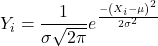
This formula has a lot of parts, but once we break down the parts, we’ll see that there is just two things to know. First, let’s identify the parts of the equation:

 is the height of the curve (normal density)
(pie) is a constant = 3.14159… (R, use pi)
µ is the population mean
σ² is the population variance
σ is the square-root of the variance or the population standard deviation
e is the natural logarithm (R, use exp())
 is the individual’s value

Why the Normal distribution is so important in classical statistics

With these distinctions out of the way, the first important message about the normal curve is that it permits us to say how likely (ie, how probable) is a particular value if the observation comes from a population with mean µ and standard deviation σ and the population from which the sample was drawn came from a normal distribution.

The second message: all we need to know to recreate the normal distribution for a set of data is the mean and the variance (or the standard deviation) for the population!! With just these two parameters, we can then determine the expected proportion of observations expected for each value of X. Note — we generally do not know these two because they are population parameters: we must estimate them from samples, using our sample statistics, and that’s where the first big assumption in conducting statistical analyses comes into play!!

An example for calculating the normal distribution when knowing the mean and variance

µ = 5, σ² = 10 (thus, the standard deviation, σ = 3.16)

The formula becomes

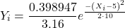
Now, plug in different values of X (for example, what’s the probability that a value of X could be 0, 1, 2, …, 10? If we really do have a normal curve with mean = 5, and variance = 10).

The normal equation returns the proportion of observations in a normal population for each X value:

When i = 5 Y₅ = 0.12616 This is the proportion of all data points that have an X = 5 When i = 1 Y₁ = 0.019995 This is the proportion of all data points that have an X = 1

We can keep going, getting the proportion expected for each value of X, then make the plot (Fig 6).

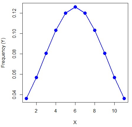
Figure 6. Frequency expected for a few points (X: 0 – 10) drawn from a normal distribution, calculated using the formula and example values. 

Here’s the R code for the plot

X = seq(0,10, by=1)
Y = (0.398947/3.16)*exp((-1*(X-5)^2)/20)
plot(Y~X, ylab="Frequency (Y)", cex=1.5, pch=19,col="blue")
lines(X,Y, col="blue", lwd=2)

Next up, more about the normal distribution, Chapter 6.7.

Questions

1. For a mean of 0 and standard deviation of 1, apply the equation for the normal curve for X = (-4, -3.5, -3, -2.5, -2, -1.5, -1, -0.5, 0, 0.5, 1, 1.5, 2, 2.5, 3, 3.5, 4). Plot your results.
2. Sample from a normal distribution with different sample size, means, and standard deviations, each time make a histogram and compare the shape of the histograms.
3. For  a subset of

Quiz Chapter 6.6

Continuous distributions

Start Quiz

Question

✕

✓

Your answer:

Correct answer:

Next

Please wait..

↺

You got {{SCORE_CORRECT}} out of {{SCORE_TOTAL}}

Your Answers

Chapter 6 contents

• Introduction
• Some preliminaries
• Ratios and proportions
• Combinations and permutations
• Types of probability
• Discrete probability distributions
• Continuous distributions
• Normal distribution and the normal deviate
• Moments
• Chi-square distribution
• t distribution
• F distribution
• References and suggested readings

6.4 – Types of probability

Introduction

By probability, we mean a number that quantifies the uncertainty associated with a particular event or outcome. If an outcome is certain to occur, the probability is equal to 1; if an outcome cannot happen, the probability is equal to zero. Most events we talk about in biology have probability somewhere in between.

A basic understanding, or at least an appreciation for probability is important to your education in biostatistics. Simply put, there is no certainty in biology beyond simple expectations like Benjamin Franklin’s famous quip about “death and taxes…”

Discrete probability

You are probably already familiar with discrete probability. For example, what is the probability that a single toss of a fair coin will result in a “heads?” The outcomes of the coin toss are discrete, categorical, either “heads” or “tails.”

And for ten tosses of the coin? And more cogently, what is the probability that you will toss a coin ten times and get all ten “heads?” While different in tone, these are discrete outcomes. An important concept is independence. Are the multiple events independent? In other words, does the toss of coin on the first attempt affect the toss of the coin on the second attempt and so on up to the tenth toss? At least in principle the repeated tosses are independent so to find the probability you just multiply each event’s probability to get the total.

In contrast, if one or more events are not independent but somehow influence the behavior of the next event, then you add the probabilities for each dependent event. We can do better than simply multiply or add events one at a time; depending on the number of discrete outcomes it is very likely that someone has already calculated all possible outcomes and come up with an equation. In the case of the tossing of two coins this is a binomial equation problem and repeat tosses can be modeled by use of the Bernoulli distribution.

Now, try this on for size. What is the probability that the next child born at Kapiolani Medical Center in Honolulu will be assigned female?

We just described a discrete random variable, which can only take on discrete or “countable” numbers.  This distribution of values is the probability mass function. The probability of a one fatal airline accident in a year exactly on 20.1 is practically zero (the area under a point along the curve is zero), so we can get the probability of a range of values around the point as our answer.

Continuous probability

Many events in biology are of degree, not kind. It is kind of awkward to think about it, but for a sample of adult house mice drawn from a population, what is the probability of obtaining a mouse that is 20.0000 grams (g) in weight? Each possible value of body mass for a mouse is considered an event, just like in our example of tossing a coin. But clearly, we don’t expect to get a lot of mice that are exactly 20.0000 g in weight. For variables like body mass, the type of data we collect is continuous, and the probability values need to be rethought along a continuum of possible values and, in turn, how likely each value is for a mouse. Although it is theoretically possible that a mouse could weigh ten pounds, we know by experience that this is impossible. Adult mice weigh between 15 and 50 g or there about.

We just described a continuous random variable, which can take on any value between a specific interval of values. This distribution of values is the probability density function (PDF). The probability of a mouse’s weight falling exactly on 20.1 is practically zero (the area under a point along the curve is zero), so we can get the probability of a range of values around the point as our answer.

In statistical inference, following our measurements of the variables from our sample drawn from a population, we make conclusions with the following kind of caveat: “the mean body mass for this strain of mouse is 20 g.” That is our best estimate of the mean (middle) for the population of mice, more specifically, for the body mass of the mice. Here, the variable body mass is more formally termed a random variable. This implies that there is in fact a true population mean body mass for the mice and that any deviations from that mean are due to chance.

In statistics we don’t settle for a single point estimate of the population mean. You will find most reporting of estimates of random variables is accompanies by a statement like, the mean was 20g with a 95% probability that the true population mean is between 18.9 and 21 g. This is called the 95% confidence interval for the mean and it takes into account how good of an estimate our sample is likely to be relative to the true population value. Not only are we saying that we think the population mean is 20g, but we’re willing to say that we are 95% certain that the true value must be between a lower limit (18.9 g) and and upper limit (21 g). In order to make this kind of statement we have to assume a distribution that will describe the probability of mouse weights. For many reasons we usually assume a normal distribution. Once we make this assumption we can calculate how probable a particular weight is for a mouse.

We introduced how to calculate Confidence Intervals in Chapter 3.4 and will extend this in any chapter that introduces an estimation.

Types of probability

To begin refining our concept of probability, it is sometimes useful to distinguish among kinds of probabilities:

• between theoretical and empirical;
• between subjective and objective.

In most cases, including your statistics book, we would begin our discussion of probability by talking of some probabilities for events we’re familiar with.

1. The theoretical probability of heads appearing the next time you flip a fair coin is 1/2 or 50%. As long as we’re talking about a fair coin, the probability of a heads appearing each time you flip the coin remains 50%. We can check this by conducting and experiment: out of 10 tosses, how many heads appear? The answer would be an empirical probability, and we understand the chance in an objective manner (no interpretation needed).
2. The theoretical probability that a “5” will appear on the face of a fair dice after a toss is 1/6 or 16.667%. Again, as long as we’re talking about a fair dice, the probability of a “5” appearing each time you roll the dice remains 16.667%.
3. The probability that at birth, a human baby’s sex will be male about 1/2 or 50%. This is an empirical probability based on millions of observations. Changes in technology, and ethical standards notwithstanding, the probability will remain the same.
4. The probability of the birth of a Downs syndrome baby is 1/800, but increases with age until by age 45, the chance is 1/12. Again, these are empirical and objective.
5. The probability of winning the Publisher’s Clearing House Sweepstakes is about 1 in 100 million. This probability is theoretical, it is also objective; however, by adding lots of twists to the game, by having multiple opportunities and by giving the appearance that a person must purchase a magazine, some players perceive their chances as increasing or decreasing by their efforts (=subjective).

R and distributions

R offers access to many named distributions. R generally provides four functions available for each.

density (d):the probability density function (PDF) for continuous distributions or the probability mass function (PMF) for discrete distributions.

probability (p): the cumulative distribution function (CDF), which is the chance (probability) of a random variable being less than or equal to a given value

quantile (q): the quantile function (inverse CDF), which returns the value at a given probability

r: draw random numbers from the specified distribution.

Examples of functions for the normal distribution then, are: dnorm(), pnorm(), qnorm(), and rnorm().

Coding example: Find the PDF for x = 0 in a standard normal distribution. # Find the PDF value for x = 0 in a standard normal distribution (mean=0, sd=1)

dnorm(x = 0, mean = 0, sd = 1)

R output

0.398942280401433

Thus, we conclude the chance that x = 0 is about 40%.

Coding example: Find the probability that for x is equal to -1.2 or less in a standard normal distribution.

pnorm(q = -1.2, mean = 0, sd = 1, lower.tail = TRUE)

R output

0.115069670221708

Thus, we conclude the chance that x is equal to or less than -1.2 is about 11.5%.

Coding example: Assuming normal distribution of test scores, what score will 50% of students score? Find the probability that for x is equal to -1.2 or less in a standard normal distribution.

qnorm(0.5, mean = 75, sd = 10)

R output

75

As expected, at 50% it returns the mean. Now, confirm that the lower 25% and upper 75% are 68.26 and 81.75, respectively.

Last coding example, draw random sample of three scores from the same exam.

rnorm(3, mean = 75, sd = 10)

R output

1. 66.0384856946112

2. 69.1887923903669

3. 77.6342297053815

R Commander: Distributions menus give four options

• Quantiles
• Probabilities
• Plot
• Sampling

Questions

1. Define and distinguish, with examples

1. discrete and continuous probability
2. theoretical and empirical probability
3. subjective and objective probability

Quiz Chapter 6.4

Types of probability

Start Quiz

Question

✕

✓

Your answer:

Correct answer:

Next

Please wait..

↺

You got {{SCORE_CORRECT}} out of {{SCORE_TOTAL}}

Your Answers

Chapter 6 contents

• Introduction
• Some preliminaries
• Ratios and proportions
• Combinations and permutations
• Types of probability
• Discrete probability distributions
• Continuous distributions
• Normal distribution and the normal deviate
• Moments
• Chi-square distribution
• t distribution
• F distribution
• References and suggested readings

5.5 – Importance of randomization in experimental design

Introduction

If the goal of the research is to make general, evidenced-based statements about causes of disease or other conditions of concern to the researcher, then how the subjects are selected for study directly impacts our ability to make generalizable conclusions. The most important concept to learn about inference in statistical science is that your sample of subjects upon which all measurements and treatments are conducted, ideally should be a random selection of individuals from a well-defined reference population.

The primary benefit of random sampling is that it strengthens our confidence in the links between cause and effect. Often after an intervention trial is complete, differences among the treatment groups will be observed. Groups of subjects who participated in sixteen weeks of “vigorous” aerobic exercise training show reduced systolic blood pressure compared to those subjects who engaged in light exercise for the same period of time (Cox et al 1996). But how do we know that exercise training caused the difference in blood pressure between the two treatment groups? Couldn’t the differences be explained by chance differences in the subjects? Age, body mass index (BMI), overall health, family history, etc?

How can we account for these additional differences among the subjects? If you are thinking like an experimental biologist, then the word “control” is likely coming to the foreground. Why not design a study in which all 60 subjects are the same age, the same BMI, the same general health, the same family … history…? Hmm. That does not work. Even if you decide to control age, BMI, and general health categories, you can imagine the increased effort and cost to the project in trying to recruit subjects based on such narrow criteria. So, control per se is not the general answer.

If done properly, random sampling makes these alternative explanations less likely. Random sampling implies that other factors that may causally contribute to differences in the measured outcome, but themselves are not measured or included as a focus of the research study, should be the same, on average, among our different treatment groups. The practical benefits of proper random sampling is that recruiting subjects gets easier — fewer subjects will be needed because you are not trying to control dozens of factors that may (or may not!) contribute to differences in your outcome variable. The downside to random sampling is that the variability of the outcomes within your treatment groups will tends to increase. As we will see when we get to statistical inference, large variability within groups will make it less likely that any statistical difference between the treatment groups will be observed.

Demonstrate the benefits of random sampling as a method to control for extraneous factors.

The study reported by Cox et al included 60 obese men between the ages of 20 and 50. A reasonable experimental design decision would suggest that the 60 subjects be split into the two treatment groups such that both groups had 30 subjects for a balanced design. Subjects who met all of the research criteria and who had signed the informed consent agreement are to be placed into the treatment groups and there are many ways that group assignment could be accomplished. One possibility, the researchers could assign the first 30 people that came into the lab to the Vigorous exercise group and the remaining 30 then would be assigned to the Light exercise group. Intuitively I think we would all agree that this is a suspect way to design an experiment, but more importantly, why shouldn’t you use this convenient method?

Just for argument’s sake, imagine that their subjects came in one at a time, and, coincidentally, they did so by age. The first person was age 21, the second was 22, and so on up to the 30th person who was 50. Then, the next group came in, again, coincidentally in order of ascending age. If you calculate the simple average age for each group you will find that they are identical (35.5 years). On the surface, this looks like we have controlled for age: both treatment groups have subjects that are the same age. A second option is to sort the subjects into the two treatment groups so that a 21 year old is in Group A, and the other 21 year old is in Group B, and so on. Again, the average age of Group A subjects and of Group B subjects would be the same and therefore controlled with respect to any covariation between age and change in blood pressure. However, there are other variables that may covary with blood pressure, and by controlling one, we would need to control the others. Randomization provides a better way.

I will demonstrate how randomization tends to distribute the values in such a way that the groups will not differ appreciably for the nuisance variables like age and BMI differences and, by extension, any other covariable. The R work is attached following the Reading list. The take-home message: After randomly selecting subjects for assignment to the treatment groups, the apparent differences between Group A and Group B for both age and BMI are substantially diminished. No attempt to match by age and by BMI is necessary. The numbers are shown in the table and then in two graphics (Fig 1, Fig 2) derived from the table.

Table 1. Mean age and BMI for subjects in two treatment groups A and B where subjects were assigned randomly or by convenience to treatment groups.

Group	Random assignment of subjects to treatment groups	Convenience assignment of subjects to treatment groups
A	35.2	28
B	35.8	43
A	32.49	28.99
B	32.87	37.37

Just for emphasis, the means from Table 1 are presented in the next two figures (Fig 1 and Fig 2).

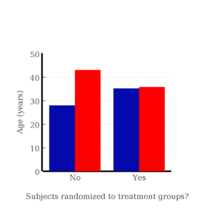
Figure 1. Age of subjects by groups (A = blue, B = red) with and without randomized assignment of subjects to treatment groups.

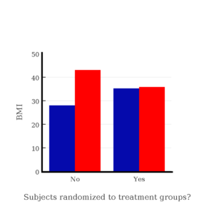
Figure 2. BMI of subjects by groups (A = blue, B = red) with and without randomized assignment of subjects to treatment groups.

Note that the apparent difference between A and B for BMI disappear once proper randomization of subjects was accomplished. In conclusion, a random sample is an approach to experimental design that helps to reduce the influence other factors may have on the outcome variable (eg, change in blood pressure after 16 weeks of exercise). In principle, randomization should protect a project because, on average, these influences will be represented randomly for the two groups of individuals. This reasoning extends to unmeasured and unknown causal factors as well.

This discussion was illustrated by random assignment of subjects to treatment groups. The same logic applies to how to select subjects from a population. If the sampling is large enough, then a random sample of subjects will tend to be representative of the variability of the outcome variable for the population and representative also of the additional and unmeasured cofactors that may contribute to the variability of the outcome variable.

What about observational studies? How does randomization work?

However, if you do cannot obtain a random sample, then conclusions reached may be sample-specific, biased. …perhaps the group of individuals that likes to exercise on treadmills just happens to have a higher cardiac output because they are larger than the individuals that like to exercise on bicycles. This nonrandom sample, an example of confounding where an extraneous or nuisance variable, body size, is associated with both the independent variable (exercise preference) and the dependent variable (cardiac output), will bias your results and can lead to incorrect interpretation of results.

Alternatively, perhaps a researcher elects to study the cardiac output of treadmill users versus bicycle users. The researcher sets up their testing station inside a gym’s powerlifting zone, where the largest individuals in the gym hang out. Inevitably because of this choice, the researcher over recruits larger individuals into the treadmill group, leading to a falsely elevated average cardiac output for treadmill users. This is an example of ascertainment bias — the sample is not representative of all treadmill users at the gym.

Random sampling is CRUCIAL in epidemiology, opinion survey work, most aspects of health, drug studies, medical work with human subjects. It’s difficult and very costly to do… so most surveys you hear about, especially polls reported from Internet sites, are NOT conducted using random sampling (included in the catch-all term “probability sampling“)!! As an aside, most opinion survey work involves complex sample designs involving some form of geographic clustering (eg, all phone numbers in a city, random sample among neighborhoods).

Random sampling is the ideal if generalizations are to be made about data, but strictly random sampling is not appropriate for all kinds of studies. Consider the question of whether or not EMF exposure is a risk factor for developing cancer (Pool 1990). These kinds of studies are observational: at least in principle, we wouldn’t expect that housing and therefore exposure to EMF is manipulated (cf. discussion Walker 2009). Thus, epidemiologists will look for patterns: if EMF exposure is linked to cancer, then more cases of cancer should occur near EMF sources compared to areas distant from EMF sources. Thus, the hypothesis is that an association between EMF exposure and cancer occurs non-randomly, whereas cancers occurring in people not exposed to EMF are random. Unfortunately, clusters can occur even if the process that generates the data is random.

Compare Graph A and Graph B (Fig 3). One of the graphs resulted from a random process and the other was generated by a non-random process. Note that the claim can be rephrased about the probability that each grid has a point, eg, it’s like Heads/Tails of 16 tosses of a coin. We can see clusters of points in Graph B; Graph A lacks obvious clusters of points — there is a point in each of the 16 cells of the grid. Although both patterns could be random, the correct answer in this case is Graph B.

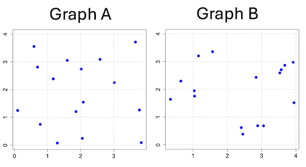
Figure 3. An example of clustering resulting from a random sampling process (Graph B). In contrast, Graph A was generated so that a point was located within each grid.

Hard to tell — and truth be told, random process could generate either one. To convince you, Figure 4 reveals the grouping that was done for Group A, in contrast with Group B which was drawn with the truly random process.

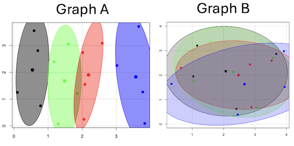
Figure 4. Same graphs as Figure 3, but with ellipses around the grouped data (hard to tell, but the centroids are the larger points). 

Implications for sampling

The graphic below shows the transmission grid in the continental United States (Fig 5). How would one design a random sampling scheme overlaid against the obviously heterogeneous distribution of the grid itself? If a random sample was drawn, chances are good that no population would be near a grid in many of the western states, but in contrast, the likelihood would increase in the eastern portion of the United States where the population and therefore transmission grid is more densely placed.

Figure 5. Map of electrical transmission grid for continental United States of America. Image source https://openinframap.org/#3/24.61/-101.16

For example, you want to test whether or not EMF affects human health, and your particular interest is in whether or not there exists a relationship between living close to high voltage towers or transfer stations and brain cancer. How does one design a study, keeping in mind the importance of randomization for our ability to generalize and assign causation?  This is a part of epidemiology which strives to detect whether clusters of disease are related to some environmental source. It is an extremely difficult challenge. For the record, no clear link to EMF and cancer has been found, but reports do appear from time to time (eg, report on a cluster of breast cancer in men working in office adjacent to high EMF, Milham 2004).

 

Questions

1. Use the sample() with and without replacement on the object (see help with R below)

fruit <- c("apple", "banana", "grape", "kiwi", "pear", "pineapple", "tomato")

a) set of 3

b) set of 4

2. Confirm the claim by calculating the probability of Graph A result vs Graph B result (see R script below).

Quiz Chapter 5.5

Importance of randomization in experimental design

Start Quiz

Question

✕

✓

Your answer:

Correct answer:

Next

Please wait..

↺

You got {{SCORE_CORRECT}} out of {{SCORE_TOTAL}}

Your Answers

---

R code!

Code you type is shown in red; responses or output from R are shown in blue. Recall that statements preceded by the hash # are comments and are not read by R (ie, no need for you to type them).

First, create some variables. Vectors aa and bb contain my two age sequences.

 aa = seq(21,50)
 bb = seq(21,50)

Second, append vector bb to the end of vector aa

 age = append(aa,bb)
 age           #submit the vector (variable) name to print the records for verification - looks good! 
  [1] 21 22 23 24 25 26 27 28 29 30 31 32 33 34 35 36 37 38 39 40 41 42 43 44 45 46 47 48 49 50 21 22 23 24 25 26 27 28 29 30 31 32 33 34 35 36 37
 [48] 38 39 40 41 42 43 44 45 46 47 48 49 50

Third, get the average age for the first group (the aa sequence)  and for the second group (the bb sequence). Lots of ways to do this, I made a two subsets from the combined age variable; could have just as easily taken the mean of aa and the mean of bb (same thing!).

 A = age[1:30]
 mean(A)
 [1] 35.5
 B = age[31:60]
 mean(B)
 [1] 35.5

Fourth, start building a data frame, then sort it by age. Will be adding additional variables to this data frame

 ex.random = data.frame(age)
 AO.all = sort(ex.random$age)
 AO.age           #submit the vector (variable) name to print the records for verification - looks good! 
  [1] 21 21 22 22 23 23 24 24 25 25 26 26 27 27 28 28 29 29 30 30 31 31 32 32 33 33 34 34 35 35 36 36 37 37 38 38 39 39 40 40 41 41 42 42 43 43 44
 [48] 44 45 45 46 46 47 47 48 48 49 49 50 50

Fifth, divide the variable again into two subsets of 30 and get the averages

 AO = AO.age[1:30]
 AO
  [1] 21 21 22 22 23 23 24 24 25 25 26 26 27 27 28 28 29 29 30 30 31 31 32 32 33 33 34 34 35 35
 mean(AO)
 [1] 28 
 BO = AO.age[31:60]
 BO
  [1] 36 36 37 37 38 38 39 39 40 40 41 41 42 42 43 43 44 44 45 45 46 46 47 47 48 48 49 49 50 50
 mean(BO)
 [1] 43

Sixth, create an index variable, random order without replacement

 rand.index = sample(1:60,60,replace=F)

Add the new variable to our existing data frame, then print it to check that all is well

 ex.random$rand = rand.index
 ex.random
    age rand
 1   21   43
 2   22   15
 3   23   17
 4   24   35
 5   25   19
 6   26   18
 7   27   22
 8   28   31
 9   29   12
 10  30   44
 11  31   24
 12  32    5
 13  33    2
 14  34   50
 15  35   23
 16  36   20
 17  37   41
 18  38   56
 19  39   36
 20  40    8
 21  41   45
 22  42   38
 23  43   42
 24  44   46
 25  45   16
 26  46   21
 27  47   28
 28  48   10
 29  49   32
 30  50   54
 31  21   57
 32  22   51
 33  23   27
 34  24   40
 35  25   14
 36  26   48
 37  27   26
 38  28   58
 39  29    9
 40  30   11
 41  31    4
 42  32   52
 43  33   37
 44  34   53
 45  35    6
 46  36   34
 47  37   39
 48  38    7
 49  39    1
 50  40   47
 51  41   33
 52  42   60
 53  43   49
 54  44   30
 55  45   29
 56  46   55
 57  47   13
 58  48    3
 59  49   25
 60  50   59

Seventh, select for our first treatment group the first 30 subjects from the randomized index. There are again other ways to do this, but sorting on the index variable means that the subject order will be change too.

 AR.age = ex.random[order(ex.random$rand),]     #created a new data frame to distinguish it from the presorted version "ex.random"

Print the new data frame to confirm that the sorting worked. It did. we can see that the rows have been sorted by ascending order based on the index variable.

 AR.age
    age rand
 49  39    1
 13  33    2
 58  48    3
 41  31    4
 12  32    5
 45  35    6
 48  38    7
 20  40    8
 39  29    9
 28  48   10
 40  30   11
 9   29   12
 57  47   13
 35  25   14
 2   22   15
 25  45   16
 3   23   17
 6   26   18
 5   25   19
 16  36   20
 26  46   21
 7   27   22
 15  35   23
 11  31   24
 59  49   25
 37  27   26
 33  23   27
 27  47   28
 55  45   29
 54  44   30
 8   28   31
 29  49   32
 51  41   33
 46  36   34
 4   24   35
 19  39   36
 43  33   37
 22  42   38
 47  37   39
 34  24   40
 17  37   41
 23  43   42
 1   21   43
 10  30   44
 21  41   45
 24  44   46
 50  40   47
 36  26   48
 53  43   49
 14  34   50
 32  22   51
 42  32   52
 44  34   53
 30  50   54
 56  46   55
 18  38   56
 31  21   57
 38  28   58
 60  50   59
 52  42   60

Eighth, create our new treatment groups, again of n = 30 each, then get the means ages for each group.

 AR = AR.age$age[1:30]
 mean(AR)
 [1] 35.16667
 AR2 = AR.all$all[31:60]
 mean(AR2)
 [1] 35.83333

Get the minimum and maximum values for the groups

 min(AR)
 [1] 22
 min(AR2)
 [1] 21
 max(AR)
 [1] 49
 max(AR2)
 [1] 50

Ninth, create a BMI variable drawn from a normal distribution with coefficient of variation equal to 20%. The first group with we will call cc

 cc = rnorm(n=30,m=27.5, sd=5.5)          #mean was 27.5 for this group with standard deviation of 5.5

The second group called dd

 dd = rnorm(n=30,m=37.5, sd=7.5)          #mean was 37.5 for this group with standard deviation of 7.5

Create a new variable called BMI by joining cc and dd

 BMI=append(cc,dd)
 BMI            #print out BMI to confirm. Looks good!
  [1] 27.87528 27.83250 31.88703 34.99041 24.06751 23.50952 22.57779 31.48394 31.04321 25.60258 25.41081 22.34619 34.62213 36.41348 41.17740
 [16] 20.56529 27.25238 21.85205 32.11690 32.37168 23.11314 33.29110 34.99106 38.22016 18.72105 26.22030 25.13412 27.50475 34.79361 32.81267
 [31] 47.57872 27.58428 40.17211 38.22195 26.91893 37.02784 53.72671 34.94727 30.35245 38.32571 40.52111 36.15627 30.36592 36.20397 47.63142
 [46] 40.30846 36.47643 50.86804 43.63741 37.84994 42.82665 41.71008 28.44976 24.57906 42.37762 38.38512 35.22879 31.34063 34.02996 27.28038

Add the BMI variable to our data frame.

 ex.random$BMI = BMI
 ex.random              #Print out the revised data frame. Looks good. We now have three variables: age, the index "rand," and now BMI
    age rand      BMI
 1   21   43 27.87528
 2   22   15 27.83250
 3   23   17 31.88703
 4   24   35 34.99041
 5   25   19 24.06751
 6   26   18 23.50952
 7   27   22 22.57779
 8   28   31 31.48394
 9   29   12 31.04321
 10  30   44 25.60258
 11  31   24 25.41081
 12  32    5 22.34619
 13  33    2 34.62213
 14  34   50 36.41348
 15  35   23 41.17740
 16  36   20 20.56529
 17  37   41 27.25238
 18  38   56 21.85205
 19  39   36 32.11690
 20  40    8 32.37168
 21  41   45 23.11314
 22  42   38 33.29110
 23  43   42 34.99106
 24  44   46 38.22016
 25  45   16 18.72105
 26  46   21 26.22030
 27  47   28 25.13412
 28  48   10 27.50475
 29  49   32 34.79361
 30  50   54 32.81267
 31  21   57 47.57872
 32  22   51 27.58428
 33  23   27 40.17211
 34  24   40 38.22195
 35  25   14 26.91893
 36  26   48 37.02784
 37  27   26 53.72671
 38  28   58 34.94727
 39  29    9 30.35245
 40  30   11 38.32571
 41  31    4 40.52111
 42  32   52 36.15627
 43  33   37 30.36592
 44  34   53 36.20397
 45  35    6 47.63142
 46  36   34 40.30846
 47  37   39 36.47643
 48  38    7 50.86804
 49  39    1 43.63741
 50  40   47 37.84994
 51  41   33 42.82665
 52  42   60 41.71008
 53  43   49 28.44976
 54  44   30 24.57906
 55  45   29 42.37762
 56  46   55 38.38512
 57  47   13 35.22879
 58  48    3 31.34063
 59  49   25 34.02996
 60  50   59 27.28038

Tenth, repeat our protocol from before: Set up two groups each with 30 subjects, calculate the means for the variables and then sort by the random index and get the new group means.

 AO = ex.random$BMI[1:30]
 mean(AO)
 [1] 28.99333
 BO = ex.random$BMI[31:60]
 mean(BO)
 [1] 37.36943

All we did was confirm that the unsorted groups had mean BMI of around 27.5 and 37.5 respectively. Now, proceed to sort by the random index variable. Go ahead and create a new data frame

 AR.age = ex.random[order(ex.random$rand),]
 AR.age                 #Print out the new data frame to confirm. Looks good.
    age rand      BMI
 49  39    1 43.63741
 13  33    2 34.62213
 58  48    3 31.34063
 41  31    4 40.52111
 12  32    5 22.34619
 45  35    6 47.63142
 48  38    7 50.86804
 20  40    8 32.37168
 39  29    9 30.35245
 28  48   10 27.50475
 40  30   11 38.32571
 9   29   12 31.04321
 57  47   13 35.22879
 35  25   14 26.91893
 2   22   15 27.83250
 25  45   16 18.72105
 3   23   17 31.88703
 6   26   18 23.50952
 5   25   19 24.06751
 16  36   20 20.56529
 26  46   21 26.22030
 7   27   22 22.57779
 15  35   23 41.17740
 11  31   24 25.41081
 59  49   25 34.02996
 37  27   26 53.72671
 33  23   27 40.17211
 27  47   28 25.13412
 55  45   29 42.37762
 54  44   30 24.57906
 8   28   31 31.48394
 29  49   32 34.79361
 51  41   33 42.82665
 46  36   34 40.30846
 4   24   35 34.99041
 19  39   36 32.11690
 43  33   37 30.36592
 22  42   38 33.29110
 47  37   39 36.47643
 34  24   40 38.22195
 17  37   41 27.25238
 23  43   42 34.99106
 1   21   43 27.87528
 10  30   44 25.60258
 21  41   45 23.11314
 24  44   46 38.22016
 50  40   47 37.84994
 36  26   48 37.02784
 53  43   49 28.44976
 14  34   50 36.41348
 32  22   51 27.58428
 42  32   52 36.15627
 44  34   53 36.20397
 30  50   54 32.81267
 56  46   55 38.38512
 18  38   56 21.85205
 31  21   57 47.57872
 38  28   58 34.94727
 60  50   59 27.28038
 52  42   60 41.71008

Get the means of the new groups

 AR = AR.age$BMI[1:30]
 mean(AR)
 [1] 32.49004
 min(AR)
 [1] 18.72105
 max(AR)
 [1] 53.72671
 AR2 = AR.all$BMI[31:60]
 mean(AR2)
 [1] 33.87273
 min(AR2)
 [1] 21.85205
 max(AR2)
 [1] 47.57872

That’s all of the work!

Data set

nonrandom

X	Y
0.779	0.747
0.098	1.248
0.697	2.811
0.59	3.553
1.295	0.075
1.858	1.207
1.172	2.388
1.597	3.051
2.051	0.242
2.081	1.546
2.016	2.738
2.587	3.088
3.833	0.088
3.776	1.264
3.017	2.254
3.657	3.712

random

X1	Y1
1.157	3.203
2.407	0.62
1.033	1.946
3.676	2.866
3.57	2.703
3.056	0.685
1.568	3.355
1.041	1.753
0.643	2.295
2.884	0.687
3.53	2.591
2.838	2.431
3.945	1.518
0.34	1.64
2.45	0.386
3.921	2.976

---

Chapter 5 contents

• The basics explained
• Experiments
• Experimental and Sampling units
• Replication, Bias, and Nuisance Variables
• Clinical trials
• Importance of randomization in experimental design
• Sampling from Populations
• References and suggested readings