20.12 – Phylogenetically independent contrasts
Introduction
Assumption of independence among the subjects in a study, key assumption. Cross species comparisons as tests of correlated evolution of traits has a long history in biology research (Cornwallis and Griffin 2024). Methods have transitioned from observations to rigorous, phylogenetic tree-based statistical approaches (phylogenetic comparative methods), and continue to provide important analytical tools, eg., host adaptation and cross-species transmission of Covid-19 virus (Attwood et al 2022).
Comparisons among species for the association between body size and metabolic rate, for example Kleiber’s Law, are classic cases (Fig 1, after Table 2 in Kleiber 1947). We’ll use Kleiber’s data basal metabolic rate (BMR) and body mass for a collection of species to explore two phylogenetic comparative methods, PIC and PGLS.
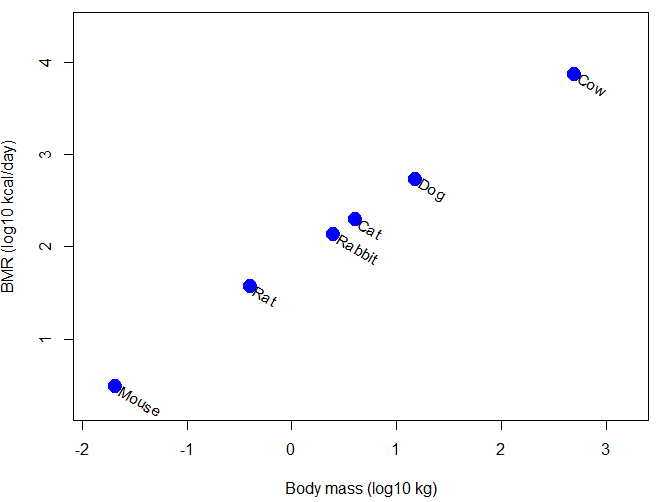
Figure 1. Scatter plot of BMR on Body Mass, log-transformed.
Typical approaches statistically, use of ANOVA or linear regression approaches. A basic assumption of ANOVA is that sampling units are independent 13.1 – ANOVA assumptions.
Prior to the 1980s, it was rarely appreciated in comparative analysis that species are not independent sample units (Harvey and Pagel 1991); evolution produced nested hierarchical relationships among the species. We recognize this with phylogenies (Felsenstein 1985, Harvey and Pagel 1991, Martins 1996, Garland et al 2005). Mice and rats share more recent common ancestor, and cattle and pigs share more recent common ancestor, than do mice and cattle, for example. Felsenstein (1985, 1988), largely credited for making the argument that Type I error likely if phylogeny ignored, and, importantly, provided an algorithm, Phylogenetic Independent Contrasts, PIC, which provided a simple way to correct for phylogenetic nonindependence. Felsentein’s landmark 1985 paper has been cited more than ten thousand times (Feb 2024).
Logic of PIC
Treating comparative data, eg, species, as a collection of independent samples implies that the evolutionary history was a spontaneous burst, or star-like phylogeny — an unresolved phylogenetic tree with branches radiating from a single ancestral node (Fig 2).
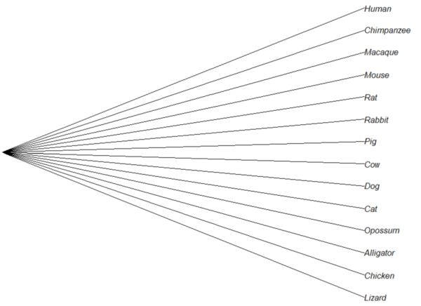
Figure 2. Star tree phylogeny (same image shown Figure 5, 20.11 – Plot a Newick tree).
But what nature provides is nonindependence (Fig 3, for more about star phylogeny in PIC see discussion in Garland et al 2005), Darwin’s “groups under groups,” or a nested hiearchy. Species are not independent units and phylogenetic history should be accounted for during statistical analysis.
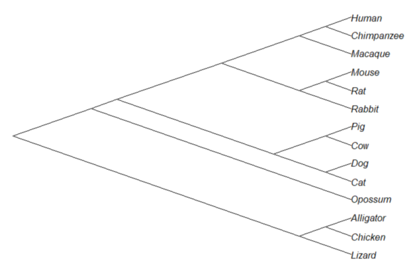
Figure 3. A cladogram for same species, showing the hierarchical, nested relationships among taxa, what nature actually provides (same image shown Figure 2, 20.11 – Plot a Newick tree).
Let’s revisit Figure 1. What do the points look like if we line up the known phylogeny for Kleiber’s six species against the plotted data? That gives us Figure 4.
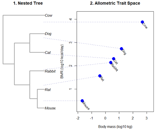
Figure 4. Kleiber’s Law and the confounding effect of shared ancestry.
Dashed connecting lines in Figure 4 trace each species from its tree position to its phenotypic value, demonstrating how phylogenetic clustering violates the independent data assumptions of standard OLS regression.
Begin R code for Figure 4, with remarks — code generated with Gemini AI assistance.
# 1. Reset the data frame
kleiber_data <- data.frame(
Species = c("Mouse", "Rat", "Rabbit", "Cat", "Dog", "Cow"),
Mass = c(0.021, 0.282, 2.45, 3.1, 13.4, 439.0),
BMR = c(3.38, 32.4, 134.0, 151.0, 506.0, 6135.0),
stringsAsFactors = FALSE
)
kleiber_data$log_Mass <- log10(kleiber_data$Mass)
kleiber_data$log_BMR <- log10(kleiber_data$BMR)

# 2. Build the exact matching standalone 6-species tree
library(ape)
newick_tree_6 <- "((((Mouse:10,Rat:10):10,Rabbit:20):20,(Cat:20,Dog:20):20):15,Cow:55);"
my_tree <- read.tree(text = newick_tree_6)

# 3. Setup a side-by-side 2-panel layout
layout(matrix(c(1, 2), nrow = 1), widths = c(1, 1.3))
par(mar = c(5, 4, 4, 1))

# PANEL 1: Plot the tree hierarchy
plot(my_tree, main = "1. Nested Tree",
edge.width = 3, edge.color = "darkgrey", cex = 1.1)

# FIXED COORDINATE MAP: 'ape' plots leaves bottom-to-top exactly matching the tree order
# We map the tree tip labels to simple integers 1 through 6
tree_heights <- 1:6
names(tree_heights) <- my_tree$tip.label

# PANEL 2: Plot the scatterplot
plot(kleiber_data$log_BMR ~ kleiber_data$log_Mass,
pch = 19, cex = 2, col = "blue",
xlab = "Body mass (log10 kg)", ylab = "BMR (log10 kcal/day)",
xlim = c(min(kleiber_data$log_Mass) - 0.2, max(kleiber_data$log_Mass) + 0.6),
ylim = c(min(kleiber_data$log_BMR) - 0.3, max(kleiber_data$log_BMR) + 0.3),
main = "2. Allometric Trait Space")

# Re-apply your custom 310-degree slanted text labels
text(kleiber_data$log_Mass + 0.05, kleiber_data$log_BMR - 0.03,
labels = kleiber_data$Species, srt = 310, adj = 0, cex = 0.9, col = "black")

# 4. CROSS-PANEL LINE CORRECTION: Draw lines across the margins safely
par(xpd = NA) # Tells R to ignore the borders of the active scatterplot window

# Calculate the left-hand margin boundaries based on the current plot limits
left_x_boundary <- min(kleiber_data$log_Mass) - 2.8

for(i in 1:nrow(kleiber_data)) {
sp <- kleiber_data$Species[i]

# A. Use a standardized geometric multiplier to align with Panel 1's vertical axis
# This formula maps the tree heights (1-6) into the scatterplot's Y coordinate scale
y_scale_factor <- (tree_heights[sp] - 1) / 5
y_span_range <- max(kleiber_data$log_BMR) - min(kleiber_data$log_BMR)
target_tree_y <- min(kleiber_data$log_BMR) + (y_scale_factor * y_span_range)

# B. Pull the actual coordinates of your blue dot
right_x <- kleiber_data$log_Mass[i]
right_y <- kleiber_data$log_BMR[i]

# C. Draw a clean, connecting line directly out to the dot
segments(x0 = left_x_boundary,
y0 = target_tree_y,
x1 = right_x,
y1 = right_y,
col = adjustcolor("darkblue", alpha.f = 0.3),
lty = 3, lwd = 2)
}

# Reset layout parameters back to normal
layout(1)
End R code.
Note 1. About the code for Figure 3. Ideally, we would use the function phylomorphospace (phytools package) to superimpose the nested tree and the plot of Kleiber’s data. For example, our code would look like
R code
library(phytools)
phylomorphospace(my_tree, trait_matrix,
label = "off", # Suppresses default horizontal text labels safely
xlab = "Body mass (log10 kg)",
ylab = "BMR (log10 kcal/day)",
xlim = c(min(kleiber_data$log_Mass) - 0.2, max(kleiber_data$log_Mass) + 0.6),
ylim = c(min(kleiber_data$log_BMR) - 0.3, max(kleiber_dat$log_BMR) + 0.3),
control = list(col.edge = "darkgrey", lwd = 3))
End R code.
However, the relationship is so perfect here that the tree lies flat on the regression line so we can’t see the tree for the line, hence our use of segments().
Phylogenetic Generalized Least Squares (PGLS).
However, like most innovations, PIC should not be blindly applied in all comparative analysis (eg, unreplicated evolutionary events, Uyeda et al 2018). Fundamentally, PIC is mathematically limited: it primarily handled simple two-variable correlations and required fully resolved, bifurcating evolutionary trees with known branch lengths. At about the same time, Grafen (1989) proposed that phylogenetic non-independence could be treated as a form of spatial autocorrelation — that is, near things are more related than distant things. Instead of computing data contrasts at individual tree nodes, Grafen introduced the phylogenetic regression, which used Generalized Least Squares (GLS) to alter how the regression algorithm treats the residual errors of species data. Improvements to phylogenetic regression are now collectively refered to as the Phylogenetic Generalized Least Squares (PGLS) (Rohlf 2001, Housworth et al 2004, Mazel et al 2016, Adams et al 2019).
Logic of PGLS.
In standard Ordinary Least Squares (OLS) regression, the residual error terms (ε) are assumed to be independent and identically distributed. In matrices, this error structure is represented by an identity matrix (I), where the off-diagonals are zero, implying that knowing about the trait value of a mouse reveals no information about the value for a rat or other rodent species.
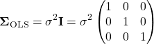
Note 2. The identity matrix  3 \times 3
 n = 3
 \sigma^{2} \times 1 = \sigma^{2}
 \sigma^{2} \times 0 = 0
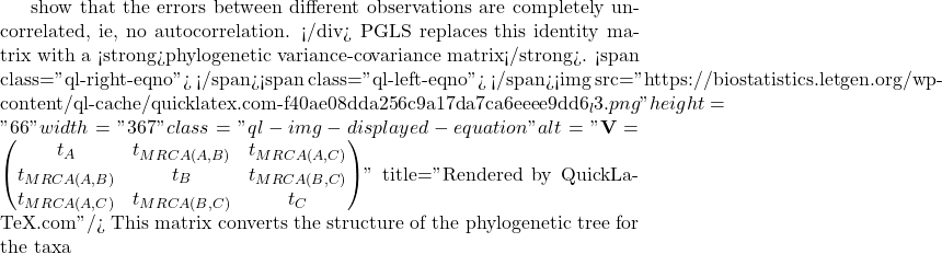
A B
 C
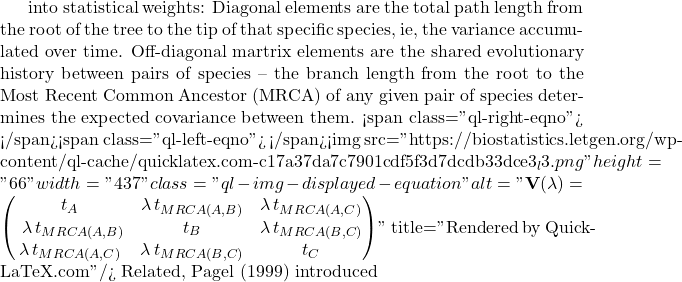
lambda Pagel’s \ \lambda
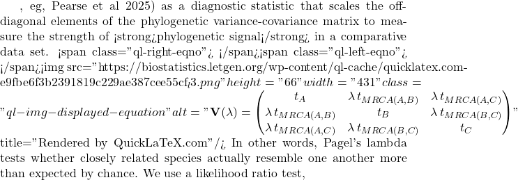
LRT \lambda

LR \chi ^{2}

\ln L_{\lambda = 0} \ln L_{\hat{\lambda}}
 \lambda
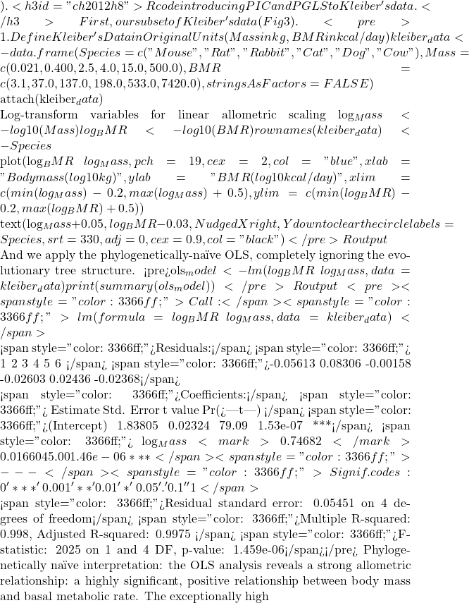 R^{2}
 BMR = aM^{b}
 \frac{3}{4}
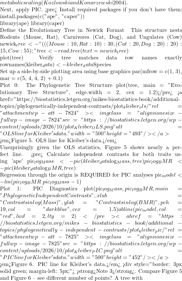 n
 n – 1
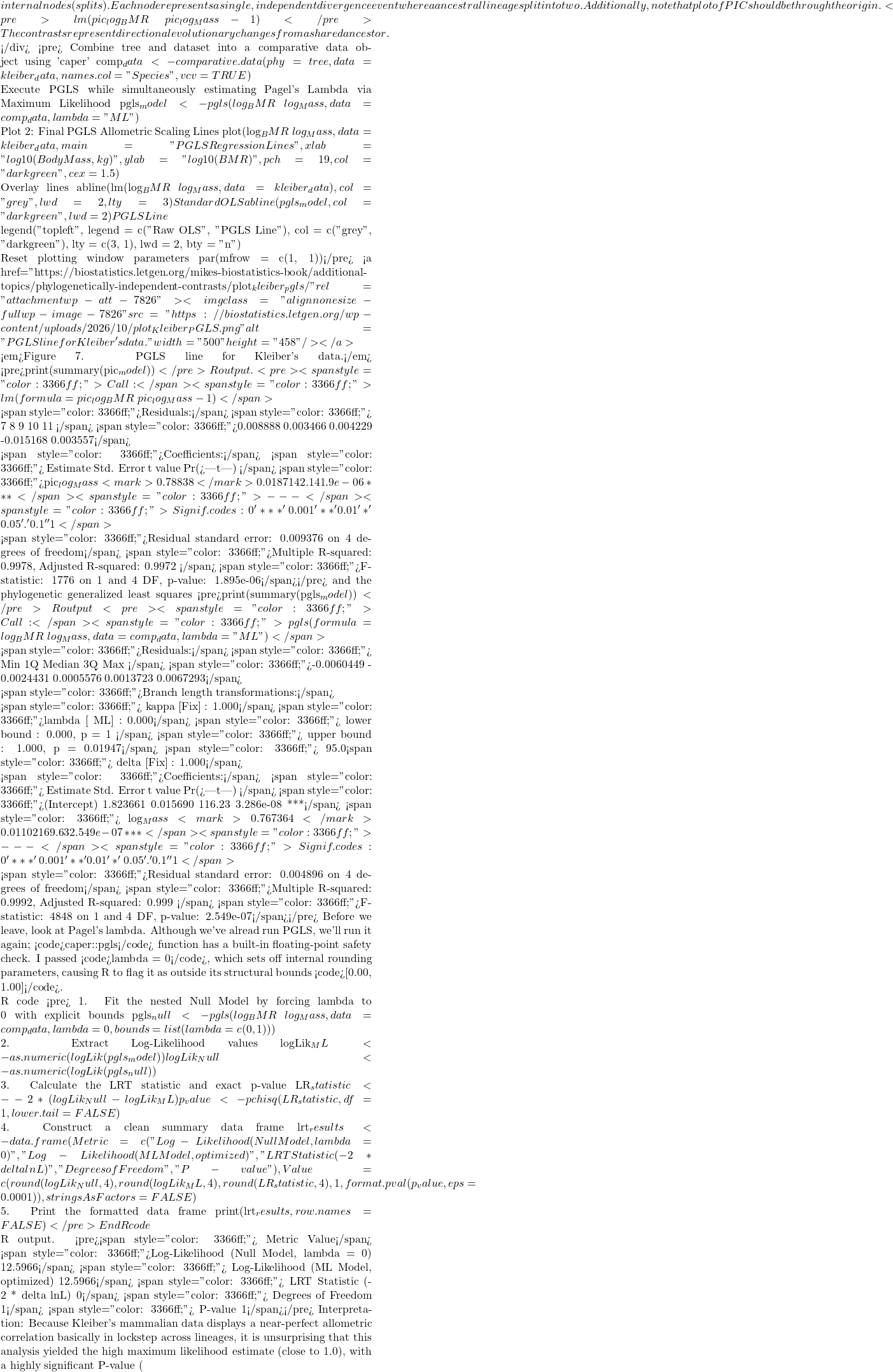 P < 0.05
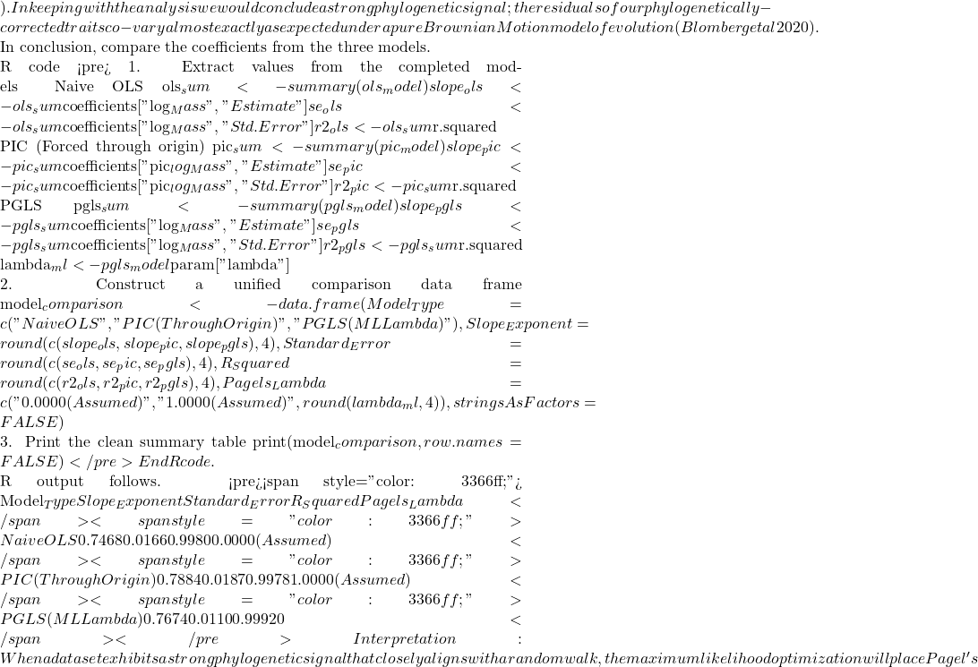 \lambda
 R^{2}$ values match identically between those two rows, while the naive OLS model stands apart due to its complete omission of tree topology.
Looking closely at the comparison of coefficients from the different models, from 0.7468 to 0.7884, it would be natural to ask, “Why go through the trouble of building a tree if the final biological answer is practically identical?” And, note that OLS and PGLS are nearly the same! The short response is only the phylogenetically correct coefficient estimates are statistically valid, and larger data sets are unlikely to reveal such agreement.
The fact that the PGLS slope (0.7674) splits the difference between the naïve OLS (0.7468) and strict PIC (0.7884) shows that Pagel’s λ converged on an intermediate value between 0 and 1. Instead of completely erasing the tree or treating it as absolute truth, PGLS multiplied the off-diagonal elements of the covariance matrix by this fractional λ value. This flattens the evolutionary branches, shrinking the expected covariance between sister taxa.
The model recognized that closely related species share some ancestral drag, but also exhibit more independent divergence than a pure random walk would predict. In contrast, the other two models represent rigid statistical boundaries:
- Naive OLS forces λ = 0, entirely ignoring the tree topology to arrive at
0.7468. - Strict PIC forces λ = 1, assuming unscaled Brownian Motion.
Because it used the full branch lengths, it shifted the trajectory heavily to 0.7884. By optimizing to an intermediate λ, PGLS strikes a perfect compromise: it protects us from the pseudoreplication of OLS while preventing the over-correction of a forced PIC.
Questions
- Mathematically, under what specific evolutionary conditions does a PGLS regression yield the exact same slope and standard error as a PIC regression?
- If your model estimates an optimized λ = 0.45, how does this physically alter the off-diagonal elements of your variance-covariance matrix compared to a standard OLS matrix?
- Why must a linear regression using Phylogenetically Independent Contrasts (PIC) be forced through the origin, omitting the standard intercept term?
- How does a PGLS matrix mathematically downweight a tight cluster of closely related species to prevent them from artificially inflating your sample size (N)?
- What happens to your Type I error rate and standard errors if you run a PGLS assuming Brownian Motion (λ = 1), but the trait actually evolved under strong stabilizing selection?
Explore on your own.
Kleiber’s data set (Table 2, 1947) contained data for humans (women) and four additional species. Redo the PIC and PGLS analysis with the updated data set. What is the effect on coefficient estimates and the standard errors with the (slightly) larger data set?
kleiber_full <- data.frame(
    Species = c("Mouse", "Rat", "Rabbit", "Macaque", "Cat", "Dog",
              "Goat", "Sheep", "Chimpanzee", "Woman", "Cow"),
# Exact body mass (W) in kilograms
    Mass = c(0.021, 0.282, 2.45, 4.20, 3.10, 13.40,
           36.00, 46.40, 38.00, 56.10, 439.00),
# Exact basal metabolic rate in kcal per 24 hours
    BMR = c(3.38, 32.7, 134.0, 207.0, 151.0, 506.0,
          826.0, 1145.0, 1090.0, 1398.0, 6135.0),
stringsAsFactors = FALSE
)
and the tree
"(((((Mouse:10,Rat:10):10,Rabbit:20):20,((Macaque:25,(Chimpanzee:6,Woman:6):19):10):10):10,(Cat:20,Dog:20):30):10,(Goat:15,Sheep:15):40,Cow:55);"
my_tree <- read.tree(text = expanded_newick)
References and suggested readings
Adams, D. C., & Collyer, M. L. (2019). Phylogenetic comparative methods and the evolution of Multivariate Phenotypes. Annual Review of Ecology, Evolution, and Systematics, 50(1):405–425.
Attwood, S. W., Hill, S. C., Aanensen, D. M., Connor, T. R., & Pybus, O. G. (2022). Phylogenetic and phylodynamic approaches to understanding and combating the early SARS-CoV-2 pandemic. Nature Reviews Genetics, 23(9), 547–562.
Blomberg, S. P., Rathnayake, S. I., & Moreau, C. M. (2020). Beyond Brownian Motion and the Ornstein-Uhlenbeck Process: Stochastic Diffusion Models for the Evolution of Quantitative Characters. American Naturalist, 195(2), 145–165.
Cornwallis, C. K., & Griffin, A. S. (2024). A guided tour of phylogenetic comparative methods for studying trait evolution. Annual Review of Ecology, Evolution, and Systematics, 55(1), 181–204.
Felsenstein, J (1985) Phylogenies and the comparative method. American Naturalist 125(1):1-15.
Felsenstein, J. (1988) Phylogenies and quantitative characters. Annual Review of Ecology and Systematics, 19, 445–471.
Garland Jr, T., Bennett, A. F., & Rezende, E. L. (2005). Phylogenetic approaches in comparative physiology. Journal of experimental Biology, 208(16), 3015-3035.
Grafen, A. (1989). The phylogenetic regression. Phil. Trans. R. Soc. London B, 326, 119-157.
Harvey, P.H. and Pagel, M.D. (1991) The Comparative Method in Evolutionary Biology. Oxford University Press, Oxford, Oxford Series in Ecology and Evolution.
Housworth, E. A., Martins, E. A. P., & Lynch, M. (2004). The phylogenetic mixed model. American Naturalist, 163, 84–96.
Kozłowski, J., & Konarzewski, M. (2004). Is West, Brown and Enquist’s model of allometric scaling mathematically correct and biologically relevant? Functional Ecology, 18(2), 283–289.
Martins, E.P. (1996) Phylogenies and the Comparative Method in Animal Behavior. Oxford University Press.
Mazel, F., Davies, T. J., Georges, D., Lavergne, S., Thuiller, W., & Peres-Neto, P. R. (2016). Improving phylogenetic regression under complex evolutionary models. Ecology, 97(2), 286–293.
Pagel, M. (1999). Inferring the historical patterns of biological evolution. Nature</i<, 401(6756), 877–884.
Paradis, E. (2012) Analysis of Phylogenetics and Evolution with R (Second Edition). New York: Springer.
Paradis, E. and Schliep, K. (2019) ape 5.0: an environment for modern phylogenetics and evolutionary analyses in R. Bioinformatics, 35, 526–528.
Pearse, W. D., Davies, T. J., & Wolkovich, E. M. (2025). How to Define, Use, and Interpret Pagel’s \ łambda \ (Lambda) in Ecology and Evolution. Global Ecology and Biogeography, 34(4), e70012.
Revell, L. J. (2012) phytools: An R package for phylogenetic comparative biology (and other things). Methods in Ecology and Evolution, 3, 217-223.
Rohlf, F. J. (2001). Comparative methods for the analysis of continuous variables: Geometric interpretations. Evolution, 55(11), 2143–2160.
Uyeda, J. C., Zenil-Ferguson, R., & Pennell, M. W. (2018). Rethinking phylogenetic comparative methods. Systematic Biology, 67(6), 1091-1109.
Zhang, J., Pei, N., & Mi, X. (2012). phylotools: Phylogenetic tools for Eco-phylogenetics. R package version 0.1, 2.
Chapter 20 contents
- Additional topics
- Area under the curve
- Peak detection
- Baseline correction
- Surveys
- Time series
- Dimensional analysis
- Estimating population size
- Diversity indexes
- Survival analysis
- Growth equations and dose response calculations
- Plot a Newick tree
- Phylogenetically independent contrasts
- How to get the distances from a distance tree
- Binary classification
- Meta-analysis
14 – ANOVA designs, multiple factors
Introduction
In our previous discussions about t-tests and ANOVA we focused on procedures with one dependent (response) variable and a single independent (predictor) factor variable that may cause variation in the response variable. In this chapter we extend our discussions about the general linear model by reviewing
- One-way ANOVA and provided a few examples of the one-way design.
- To review and set the stage for adding a second independent variable to the model.
Additional one-way ANOVA examples
1. In a plants, we may have a response variable like height and one factor variable (location: sun vs. shade) thought to influence plant height (eg, Aphalo et al 1999).
2. Pulmonary macrophage phagocytosis behavior (response variable) after exposure of toads to clean air or ozone (factor with 2 levels) (Dohm et al. 2005).
3. Monitor weight change on subjects after 6 weeks eating different diet (DASH, control) (Elmer et al. 2006).
All three of the examples are based on the same statistical model which may be written as:

where μ is the grand mean, Y is the response variable and A is the independent variable, or factor, with k = 1, 2, …. K levels, groups, or treatments. The total number of experimental units (eg, subjects) is given by i = 1, 2, 3, … n. Note that in the first and third examples, because there were only two groups (example 1: k = location, shade; example 3: k = DASH, control) note that this problem could have been evaluated as an independent sample t-test. For the second example, there were three groups so k = clean air, first ozone level, second ozone level).
Two-way ANOVA with replication
As useful as the one-way ANOVA design can be, it is a “one-factor-at-a-time” approach (Radzilani et al 2025), experiments are typically more complicated than a single t-test or one-way ANOVA design can handle; rarely would we conduct an experiment that reflects only one source of variation. Looking only at variability for one factor at a time while while keeping all other factors constant ignores interactions between factors, resulting in potentially serious model bias (eg, discussed in Vatcheva et al 2015).
For example, while diet has a profound effect on weight, clearly, activity levels are also important. At a minimum, when considering a weight loss program, we would want to control or monitor activity of the subjects. This is a two-factor model, and the main effects, the two factors, were diet (factor A) and activity, (factor B). Both are expected to affect weight loss, and, perhaps, they may do so in complicated ways — an interaction (eg, on DASH diet, weight loss is accelerated when subjects exercise regularly).

The subject of this chapter is the introduction to two-way ANOVA designs. In fact, to many, ANOVA design is practically synonymous to a statistician when they think about experimental design (Lindman 1992; Quinn and Keough 2002). As noted by Quinn and Keough (2002) in the preface to their book, “… many biological hypotheses, even deceptively simple ones, are matched by complex statistical models” (p. xv). Once you start adding factor variables there becomes a number of ways in which the groups and experimental units can be distributed, and thus impact the inferences one can make from the ANOVA results. The first statistical model we introduced was the one-way ANOVA. Next, we begin the two-way ANOVA with the crossed, balanced, fully replicated design. Along the way we introduce model symbols to help us communicate the design structure and implications of the statistical models.
Quizzes in this chapter
A total of 71 questions among the several subchapters, a mix of true or false and multiple choice question format.
Chapter 14 contents
5.2 – Experimental units, Sampling units
Introduction.
Sampling units refer to the measured items, the focus of data collection; samples are selected from populations. Often, sampling units are the same thing as individuals. For example, if we are interested in the knowing whether men are more obese than women in Hawai’i, we would select individuals from the population; we would measure individuals. Thus, the sampling unit would be individuals, and the measurement unit would be percent body fat recorded for each individual. The data set would be the collection of all body fat measures for all individuals in the study, and we would then make inferences (draw conclusions) about the differences, if any, between adult males and females for body fat.
But sampling units can also refer to something more restrictive than the individual. For example, we may be interested in how stable, or consistent, is a person’s body fat over time. If we take a body fat measure once per year over a decade on the same group of adults, then the sampling unit refers to each observation of body fat recorded (once per year, ten times for an individual), and the population we are most likely to be referring to is the collection of all such readings (ten is arbitrary — we could have potentially measured the same individual thousands of times).
In some cases the researcher may wish to compare groups of individuals and not the individuals themselves. For example, a 2001 study sought to see if family structure influenced the metabolic (glycemic) control of children with diabetes (Thompson et al 2001). The researchers compared how well metabolic control was achieved in children of single parents and two-parent families. Thus, the sampling units would be families and not the individual children.
Experimental units.
Experimental units refers to the level at which treatments are independently applied in a study. Often, but not always, treatments are applied directly to individuals and therefore the sampling units and experimental units in these cases would be the same.
Question 1: What is the sampling unit in the following cell experiment?
A technician thaws a cryo tube containing about ½ million A549 cells (Foster et al 1998) and grows the cells in a T-75 culture flask (the 75 corresponds to 75 cm2 growing area) in a CO2 incubator at 37 °C. After the cells reach about 70% confluency, which may represent hundreds of thousands of cells, the technician aliquots 1000 cells into twelve wells of a plate for a total of 12000 cells. To three wells the technician adds a cytokine, to another three wells he adds a cytokine inhibitor, and to another three wells he adds both the cytokine and it’s inhibitor, and to the last three wells he adds DMSO, which was the solvent for both the cytokine and the inhibitor. He then returns the plate to the incubator and 24 hours later extracts all of the cells and performs a multiplex quantitative PCR to determine gene expression of several target genes known to be relevant to cell proliferation.
The described experiment would be an example of a routine, but not trivial procedure the technician would do in the course of working on the project in a molecular biology laboratory.
The choices for numbers provided in the description we may consider for the number of sampling units are:
- 1000 cells
- 12,000 cells
- ½ million cells
- 3 wells
- 12 wells
- The target genes
- None of the above
The correct answer is G, None of the above.
“None of the above” because the correct answer is … there was just one sampling unit! All cells trace back to that single cryo tube.
To answer the question, start from the end and work your way back. What we are looking for is independence of samples and at what level in the experiment we find independence. Our basic choice is between numbers of cells and numbers of wells. Clearly, cells are contained in the wells, so all of the cells in one well share the same medium, being treated the same way, including all the way back to the cryo tube — all of the cells came from that one tube so this lack of independence traces all the way back to the source of the cells. Thus, the answer can’t be related to cell number. How many wells did the technician set up? Twelve total. So, the maximum number of sampling units would be twelve, unless the samples are not independent. And clearly the wells (samples) are not independent because, again, all cells in the twelve wells trace back to a single cryo tube. Thus, from both perspectives, wells and cells, the answer is actually just one sampling unit! (Cumming et al 2007; Lazic 2010). Finally, the genes themselves are the targets of our study — they are the variables, not the samples. Moreover, the same logic applies — all copies of the genes are in effect descended from the few cells used to start the population.
Experimental and sampling units often, but not always the same.
Question 2: What is the experimental unit in the described cell experiment?
- 1000 cells
- 12,000 cells
- ½ million cells
- 3 wells
- 12 wells
- The target genes
- None of the above
The correct answer is E, 12 wells. Noted above, the technician applied treatments to 12 wells. DMSO was added to all wells. There were three treatments, cytokine, inhibitor, and cytokine-inhibitor (Table 1).
Table 1. Translate experiment description to a table to better visualize the design
| Wells | Treatment |
|---|---|
| A1 | Cytokine |
| A2 | Cytokine |
| A3 | Cytokine |
| A4 | DMSO |
| B1 | Inhibitor |
| B2 | Inhibitor |
| B3 | Inhibitor |
| B4 | DMSO |
| C1 | Cytokine+Inhibitor |
| C2 | Cytokine+Inhibitor |
| C4 | Cytokine+Inhibitor |
| C4 | DMSO |
Note 1: Use package ggplate to create a simple graphic to visualize a culture plate.
table01.ch05.2 <- data.frame(
     well = c("A1", "A2", "A3", "B1", "B2", "B3", "C1",
              "C2", "C3", "A4", "B4", "C4", "D4"),
     treatment = c(rep("Cytokine", 3), rep("Inhibitor", 3),
              rep("Cytokine + Inhibitor", 3), rep("DMSO", 4))
     )
plate_plot(data = table01.ch05.2,
     position = Well,
     value = Treatment,
     plate_size = 12,
     plate_type = "round")
which results in this nice plate layout (Fig 1)

Figure 1. Plate layout for Table 1. Plot made with plate_plot() function from R package ggplate.
If observations were made, then the same function can display values. Add a column of values to the dataset (eg, “Values”), then add another value = line, eg, value = Values to the R code.
Replication: Groups and individuals as sampling units.
The correct identification of levels at which sampling independence occurs is crucial to successful interpretation of inferential statistics.
Note 2:replication in Table 1: three cytokine, three cytokine-inhibitor, three with both.
Sampling error rate is evaluated at the level of the sampling units. Technical replication of sampling units allows one to evaluate errors of measurement (eg, instrument noise) (Blainey et al 2014) and other sources of technical sources of noise.
Note 3: Data noise refers to random or irrelevant information that corrupts the “true” signal in a dataset, introducing variability and potential errors. A nuisance variable is a specific type of noise that is fundamental to the data collection process but not of interest to the researcher, and its effect must be accounted for or removed via pre-processing steps. For approaches to control for noise, see Chapter 17.4 and Chapter 20.3 for more.
Replication of sampling units increases statistical power, the ability to correctly reject hypotheses. If the correct design reflects sampling units are groups and not individuals, then by counting the individuals as the independent sampling units would lead the researcher to think his design has more replication than it actually does. The consequence on the inferential statistics is that he will more likely reject a correct null hypothesis, in other words, the risk of elevated type I error occurs (Chapter 8 – Inferential statistics). This error, confusing individual and group sampling units, is called pseudoreplication (Lazic 2010).
Consider a simpler experimental design scenario depicted in Figure 2: Three different water treatments (eg, concentrations of synthetic progestins, Zeilinger et al. 2009) in bowls A, B, and C; three fish in bowl A, three fish in bowl B, and three fish in bowl C. The outcome variable might be a stress indicator, eg, plasma cortisol (Luz et al 2008).
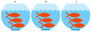
Figure 2. Three aquariums, three fish. Image modified from https://www.pngrepo.com/svg/153528/aquarium
Question 3: What were the experimental units for the fish in the bowl experiment (Fig 2)?
- Three bowls
- Nine fish
- Three water treatments
The correct answer is A, 3 bowls. The treatments were allocated to the bowls, not to individual fish. The three fish in each bowl provides technical replication for the effects of bowl A, bowl B, and bowl C, but does not provide replication for the effects of the water treatments. Adding three bowls for each water treatment, each with three fish, would be the simplest correction of the design, but may not be available to the researcher because of space or cost limitations. The design would then include nine bowls and 27 fish. If resources are not available to simply scale up the design, then the researcher could repeat the study several times, taking care to control nuisance variables (Chapter 5.3). Alternatively, if the treatments were applied to the individual fish, then the experimental units become the individual fish and the bowls reduced to a blocking effect (Chapter 14.4), where differences may exist among the bowls, but they are no longer the level by which measurements are made.
Note 4: If pseudoreplication is present in a study, then this may be accounted for by specifying the error structure in a linear mixed model (eg, random effects, blocking effects, etc., see Chapter 14 and Chapter 18).
Question 4: What were the sampling units for the fish in the bowl experiment (Fig 2)?
- Three bowls
- Nine fish
- Three water treatments
The correct answer is B, the individual fish. If instead of aqueous application of synthetic progestin, treatments were applied directly to each fish via injection, what would be the answers to Question 3 and Question 4?
Choices like these clearly involve additional compromises and assumptions about experimental design and inference about hypotheses.
Conclusion.
Sampling units, experimental units, and the concept of level at which units are independent within an experiment were introduced. Lack of independence yields the problem of pseudoreplication in an experiment, which will increase the chance that we will detect differences between our treatment groups, when no such difference exists!
Questions.

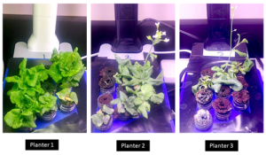
Figure 3. Three Miracle-Gro AeroGarden planters®, each with nine seedlings of an Arabidopsis thaliana strain.
Nine seeds each of three strains of Arabidopsis thaliana were germinated in three Miracle-Grow AeroGarden® hydroponic planters (Fig 3). Each planter had nine or ten vials with sphagnum peat. All seeds from a strain were planted in the same apparatus, one seed per vial. With respect to this experimental design
1. Define experimental units and sampling units.
2. Provide design examples where the experimental units are the same as the sampling units.
3. With respect to the independent and dependent (outcome) variables, discuss impacts of nuisance variables.
Quiz Chapter 5.2
Experimental units, Sampling units