20.1 – Area under the curve

Introduction
Physiology area under the curve
Machine Learning area under the curve
Area under the receiver operating carrier curve
Area under the precision recall curve
References and suggested readings
Questions
Chapter 20 contents

Introduction.

The classical physiological area under the curve, AUC, represents the total change in $y$ given change in $x$ . For example, if $x$ is time, and $y$ is oxygen consumption — eg, respirometry: recorded as an analog voltage output (millivolts or volts) from a gas analyzer to a data acquisition (DAQ) board — an AUC would be appropriate to quantify the total oxygen consumption following strenuous exercise (Excess post-exercise oxygen consumption, EPOC) or following a large meal (Specific Dynamic Action, SDA). The area represents the total, cumulative volume of oxygen consumed over that specific timeframe, eg, calculating an individual’s total EPOC.

In machince learning, the axes are probabilities and error rates. The area tells you how accurate a decision-making model is. We plot True Positive Rate (Sensitivity) against False Positive Rate (1 – Specificity) across every possible mathematical decision threshold (from 0% to 100% confidence). The curve now represents the shifting balance between catching true positives and committing false positives and the area summarizes how cleanly the model separates two distinct classes, eg, Sick vs. healthy. An area of 1.0 means perfect separation with zero overlap.

Area under the relative (receiver) operating carrier, AUROC, shows characteristics of a diagnostic model, a graphic used to show trade off between sensitivity and specificity. Classifier performance. Used to find the appropriate cut-off. Plot true positive rates against false positive rates as cumulative functions, shows the relationship between sensitivity and specificity for every possible cut off value. Can then calculate AUC to get a measure of the intervention’s ability to discriminate between true and false positive rates.

Related, area under precision-recall curve, AUPRC, is a single scalar metric that measures a binary classification model’s ability to balance precision (how many predicted positives are actually positive) and recall (how many actual positives are caught) across all possible decision thresholds. Here, precision and recall refer to both the accuracy of the model’s positive predictions and its ability to find all the positive cases.

From Chapter 7 we defined

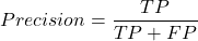
$\begin{align*} Precision = \frac{TP}{TP+FP} \end{align*}$

where $TP$ is true positives and $FP$ is false positives.

We now introduce recall, which is also refered to as sensitivity

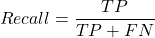
$\begin{align*} Recall = \frac{TP}{TP+FN} \end{align*}$

Precision measures the quality of your model’s positive guesses; Recall measures how many actual positive cases in the dataset were identified by the model.

AUC evaluates a model’s ability to distinguish between both $TP$ and $FP$ equally, while AUPRC focuses strictly on the model’s performance regarding the positive (rare) class.

AUC would be preferred when your dataset is balanced (equal positives and negatives) OR when you care equally about performance on both classes. For example, dataset of patients with flu or Covid from a clinic during winter months where there is roughly balanced 50/50 split of patients presenting with either Flu or Covid. You want a model that accurately classifies both which favors AUC approach.

AUPRC would be the choice when your dataset is highly imbalanced, ie, the positive class is rare. In contrast, AUPRC would be favored for scenarios where a researcher is screening 100,000 asymptomatic patients for a rare disease that only 10 people actually have.

Physiology Area under the curve

Download and install R package MESS; requires geepack, geeM, and Matrix packages

R code

x <- seq(1:10) 
y <- c(1,4,5,2,11,22,9,7,5,1) 
#length(x)==length(y)
#smooth the data 
loxy <- loess(y~x)
#Make a plot (Fig. 1)
plot(x,y, pch=19, cex=2, col="blue") 
lines(predict(loxy), type="l", col="red")

where == is an R comparison operator.

And R output

area under the curve, AOC, example

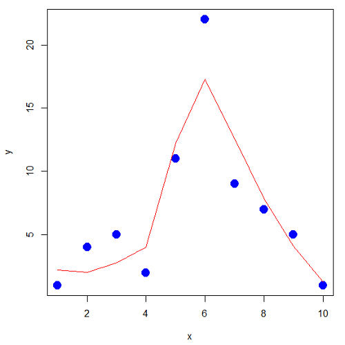
Figure 1. Area under the curve example.

library(MESS) 
auc(x,y,from=0,rule=2) 
auc(x,loxy$fitted,from=0,rule=2)

And R output

#area under curve for raw data
[1] 67
#area under curve for smoothed data
[1] 66.77616

Machine Learning area under the curve.

# Install and load the ROCR package if you haven't already
# install.packages("ROCR")
# modified from https://rviews.rstudio.com/2019/03/01/some-r-packages-for-roc-curves/

library(ROCR)
df <- data.frame(ROCR.simple)
pred <- prediction(df$predictions, df$labels)
perf <- performance(pred,"tpr","fpr")

# 1. Calculate the actual numeric AUC value
auc_perf <- performance(pred, "auc")
auc_value <- round(unlist(auc_perf@y.values), 4)

# 2. Plot the ROC curve with colorized thresholds and custom labels
plot(perf, 
colorize = TRUE, 
main = "ROC Curve",
xlab = "False Positive Rate (1 - Specificity)",
ylab = "True Positive Rate (Sensitivity)")

# 3. Add the AUC value as a subtitle
mtext(paste("AUC =", auc_value), side = 3, line = 0.5)

# 4. Add a diagonal 50/50 reference line
abline(a = 0, b = 1, lty = 2, col = "darkgray")

End R code.

Note 1. I mostly provide S3 R code examples in this eBook. In R, the @ symbol is used to extract a specific piece of data (called a slot) from an S4 object. It works almost exactly like the $ sign, but while $ is used for basic lists or standard data frames (S3 objects), @ is reserved strictly for the more structured, formal object system in R known as S4.

R output.

The calculated AUC was $0.8341875$ . The right-hand axes are color codes by AUC values (Fig 2): good tests AUC between 0.8 and 0.9, very good tests greater than 0.9.

ROC plot

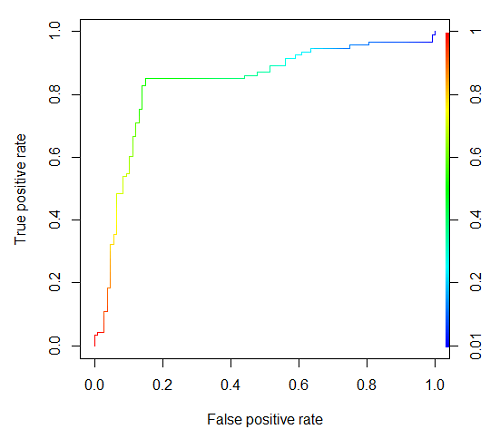
Figure 2. Example ROC curve.

Area under the precision recall curve

AUPRC measures the overall performance of a binary classification model by summarizing how well it balances precision and recall across all possible decision thresholds. A score closer to 1.0 means the model is very good at finding real positive cases without making many mistakes, which is especially useful when your dataset has very few positive examples. A score closer to 1.0 means the model is very good at finding real positive cases without making many mistakes.

R code.

library(ROCR)

# 1. Prepare data and prediction object
df <- data.frame(ROCR.simple)
pred <- prediction(df$predictions, df$labels)

# 2. Extract Precision and Recall for the plot
perf_pr <- performance(pred, measure = "prec", x.measure = "rec")

# 3. Calculate the numeric AUPRC value
# In ROCR, AUPRC is calculated by finding the Area Under the Precision/Recall curve ("aucpr")
perf_auprc <- performance(pred, measure = "aucpr")
auprc_value <- round(unlist(perf_auprc@y.values), 4)

# Print the final AUPRC score to the console
cat("The calculated AUPRC is:", auprc_value, "\n")

# 4. Plot the Precision-Recall Curve using base R graphics
plot(perf_pr, 
colorize = TRUE, 
main = paste("Precision-Recall Curve (AUPRC =", auprc_value, ")"),
xlab = "Recall (Sensitivity)", 
ylab = "Precision (Positive Predictive Value)")

End R code.

R output.

The calculated AUPRC was $0.7875$ .

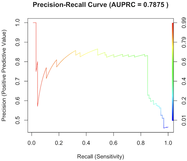
Figure 3. Precision recall curve.

The differences: AUC evaluates how well the model separates both classes equally, while AUPRC evaluates how reliably the model handles the positive class alone.

The Interpretive baselines:

Figure 2: AUC Baseline is always 0.5. A completely random model yields a diagonal line from (0,0) to (1,1), resulting in an AUC of 0.5. This baseline never changes, regardless of how rare your disease is.
Figure 3: AUPRC Baseline depends on prevalence. A random model yields a flat horizontal line across the plot. The height of this line equals the proportion of positive cases in your dataset ( $\text{Positives} / \text{Total}$ ). If only 1% of the patients have a rare condition, a random model’s AUPRC baseline is 0.01.

What a shifting threshold means:

On an AUC Curve: As you lower your decision threshold to catch more sick people, you track how fast your True Positive Rate rises compared to your False Positive Rate. You are looking at the overall trade-off between the entire healthy population and the entire sick population.
On an AUPRC Curve: As you lower your threshold to catch more sick people, you track Recall against Precision. This evaluates the quality of the “Positive” alerts. It directly measures how quickly the pool of patients you flagged as “high risk” becomes diluted with false alarms.

References and suggested readings

Çorbacıoğlu, Ş. K., & Aksel, G. (2023). Receiver operating characteristic curve analysis in diagnostic accuracy studies: A guide to interpreting the area under the curve value. Turkish Journal of Emergency Medicine, 23(4), 195–198.

Lobo, J. M., Jiménez-Valverde, A., & Real, R. (2008). AUC: A misleading measure of the performance of predictive distribution models. Global Ecology and Biogeography, 17(2), 145–151.

Martin, B., Bennett, T. D., DeWitt, P. E., Russell, S., & Sanchez-Pinto, L. N. (2025). Use of the Area Under the Precision-Recall Curve to Evaluate Prediction Models of Rare Critical Illness Events. Pediatric Critical Care Medicine, 26(6), e855–e859.

Ozenne, B., Subtil, F., & Maucort-Boulch, D. (2015). The precision–recall curve overcame the optimism of the receiver operating characteristic curve in rare diseases. Journal of Clinical Epidemiology, 68(8), 855–859. https://doi.org/10.1016/j.jclinepi.2015.02.010

Steyerberg, E. W., & Vergouwe, Y. (2014). Towards better clinical prediction models: Seven steps for development and an ABCD for validation. European Heart Journal, 35(29), 1925–1931.

Questions

Write up three learning outcomes for this page. Hint: Point your favorite generative AI to this page and ask for help

Chapter 20 contents

/MD