2.1 – Why (Bio)Statistics?
- What are the basic elements of biostatistics? .
- Why we require you to take Biostatistics as part of your major?.
- But, I’m pre-med and plan to apply to medical school ….
- With machine learning and AI, why learn biostatistics?.
- In what disciplines are biostatisticians employed?.
- Conclusions.
- Questions.
- Quiz.
- Chapter 2 contents
What are the basic elements of biostatistics?
.
What will you learn from an introductory course on (bio)statistics? Concepts and skills: An understanding (concepts) about the purpose and limits of descriptive statistics, inferential statistics, and statistical modeling for answering questions in biology and how to use elements of R programming (skills) applied to biology-related data sets to accomplish these tasks (see Table 1). Related, you will learn how (skills) to collect and manage data from projects, and why (concepts) statistical analysis can help answer questions, even inform decisions in public health. Thus, assessment in BI-311 of student learning includes both formative and summative assignments, exams, and culminates with a student research project.
Note 1: From time to time in this book I write “(bio)statistics” instead of “biostatistics.” It’s my subtle way of highlighting that whatever argument or statement is attached applies more generally to the statistical discipline, not just biostatistics. However, I’m not particularly consistent with this typology in the book.
What skills are you going to get from all of this? You will get different opinions on the elements of an essential first course in statistics or biostatistics. Certainly the basics are a foundation in probability and a breadth of classical elementary statistical procedures, which will include descriptive statistics, analysis of variance and linear regression, and an introduction to multivariate analysis. In preparation for your course in epidemiology you will also be introduced to risk analysis and survival analysis. However, the primary return for your time, I hope, will be a deeper appreciation for how to think about problems in biology from experimental design and data analysis perspectives. Practical skills you will learn include how to process and clean data for analysis, data visualization, and a foundation in parametric and nonparametric statistical methods.
The data sets described and provided in this course are small, with sample sizes in the tens to thousands (rarely). This framework is consistent with the development of the discipline of (bio)statistics, which originated to help interpret experiments conducted in agriculture, industry, and medical research (see Chapter 2.3). But, as you now know, because of genomics and other data-intensive disciplines, data sets can be very large, much beyond the kinds of data sets used prior to use of the computer in data analysis. However, as we will argue later on this page, learning foundational skills in (bio)statistics with small data sets facilitates working with and gaining insights from larger data sets. For example, we will emphasize during our work this semester how to develop a workflow with small data sets; these same workflows then can be scaled up and would include pipelines — based on tools and techniques developed in the broader discipline of bioinformatics — to large data sets, including use of Artificial Intelligence and machine learning.
Note 2: In data science, a workflow refers to the entire, end-to-end process needed in a project, from data collection, data processing, to descriptive statistics and modeling or inferential statistics, and report writing. A pipeline described elements of a workflow that can be automated.
Why we require you to take (Bio)statistics as part of your major?
.
At Chaminade University we require all biology students to take biostatistics, and we do so with an emphasis on use of data analysis skill development. This requirement aligns our program to national expectations of biology undergraduate education (eg, AAAS, NAS, NIH, NSF). As stated in Bio2010: Transforming Undergraduate Education for Future Research Biologists,
“Biology majors should be adept at using computers to acquire and process data, carry out statistical characterization of the data and perform statistical tests, and graphically display data in a variety of representations (p. 15).”
Learning biostatistics from a course like BI311 — which relies heavily on use of the R programming language and data sets — helps the biology student develop these skills.
In the next pages I will outline a history of statistics (Chapter 2.3), but here I wish to make the point that biostatistics is now considered to be a core skill set for biologists. Biostatistics as a discipline came into its own in the 1930’s, but extensive reliance on statistics in research really dates to more recent times because of the ubiquity of personal computers (Salsburg 2002). Modern biological and biomedical research requires computational and quantitative methods to collect, process, analyze, and interpret large data sets. And yet, even a casual survey of required courses for entry into graduate programs in biology (eg, only recommended for admissions to Marine Biology and Cell and Molecular Biology programs at University of Hawaiʻi – Manoa) will reveal that biostatistics is not required of candidates; so, what gives?
The first point is that programs list only minimum requirements. The second point is that many programs (genomics, ecology, etc) will expect the graduate student to take a year or more of (bio)statistics. The need is so crucial that at Harvard Medical School, all biology graduate students are expected to take a crash-course in computing and statistics to work with data (Stefan et al 2015).
Moreover, while graduate programs are not listing statistics as a requirement, many biology undergraduate curricula now require a course in (bio)statistics to reflect the increasingly data driven modern biology — where the jobs are!
My BI-311 students, I’ll make you a bet — or at least, I’ll make this part of your required homework (see BI311 Workbook)! Even a causal search of a research journal article in a biology discipline of your choosing will prove that there is no doing biology research today without an understanding of statistics.
But, I’m pre-med and plan to apply to medical school …
.
Even a cursory look at the literature will result in finding many authors strongly calling for this kind of preparation for a successful career in medicine (eg, Brieger and Hardin 2012). It’s obvious, but needs stating — you’re applying to medical school to become a doctor — you’ll spend the majority of your adult life as a doctor. Statistical thinking is crucial to answering the daily question: “My patient tested positive for biomarker X, what’s the chance that the patient has disease Y?”
Note 3: Following work done by Biomarkers and Surrogate Endpoint Working Group (Clin. Pharmacol. Ther. 69(3), 89–95 2001), biomarkers are biological characteristics that can be “… objectively measured and evaluated as an indicator of normal biological processes, pathogenic processes, or pharmacological responses to a therapeutic intervention” (Naylor 2003). Compare to biomarkers are “[a] defined characteristic that is measured as an indicator of normal biological processes, pathogenic processes, or responses to an exposure or intervention, including therapeutic interventions” (2016 by FDA-NIH Biomarker Working Group in BEST (Biomarkers, EndpointS, and other Tools) Resource).
If your answer today is, the patient has the disease, then you objectively need this course! Hint: there are four possible outcomes, not two, of a test, see Chapter 7.3 – Conditional Probability and Evidence Based Medicine.
Need more convincing? Take a look at the targets of questions intended to evaluate Skill 4 of the Scientific Inquiry and Reasoning Skills standard of the revised MCAT2015 Exam (p. 107, What’s on the MCAT2015 exam?).
- Using, analyzing, and interpreting data in figures, graphs, and tables.
- Evaluating whether representations make sense for particular scientific observations and data.
- Using measures of central tendency (mean, median, and mode) and measures of dispersion (range, interquartile range, and standard deviation) to describe data.
- Reasoning about random and systematic error.
- Reasoning about statistical significance and uncertainty (eg, interpreting statistical significance levels, interpreting a confidence interval).
- Using data to explain relationships between variables of make predictions.
- Using data to answer research questions and draw conclusions.
- Identifying conclusions that are supported by research results.
- Determining the implications of results for real-world situations.
Before we move on, there’s another justification for learning biostatistics we need to discuss.
With machine learning and AI, why learn biostatistics?
Oh, my goodness. If I was starting over, I would definitely want to pursue expertise in machine learning, ML (Fig 2). Machine learning is about finding patterns in large data sets, and modern biological research may be characterized by the impact of large datasets. The machine learning field, and artificial intelligence, AI, in general, are rapidly evolving, but built on more than 20 years of algorithm and computer discoveries. So why not skip biostatistics and go directly to data science?
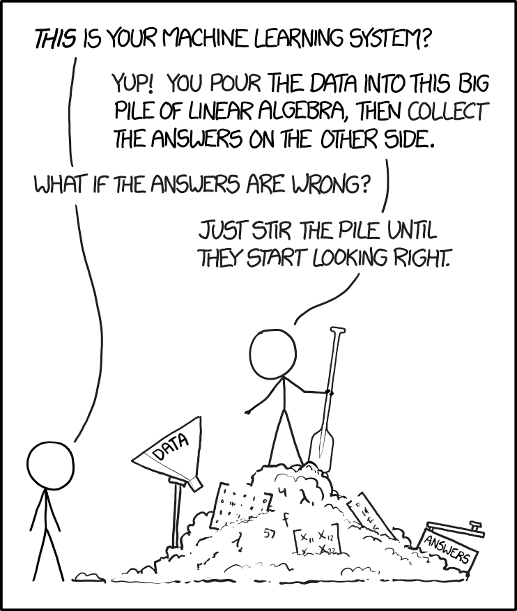
Figure 2. “Machine learning,” https://xkcd.com/1838/.
The parable presented in Figure 2 is about right: Without understanding the statistical foundations behind machine learning algorithms, you’re using tools without really knowing how they work (Lin et al 2025, more generally, see Downey 2024). We have a lot of work ahead of us, but, from time to time, we will exploit the power of AI and ML. For a start, I asked ChatGPT (August 2025), “What statistics is most relevant for ML?”, AI listed responses mapped to “Mike’s Biostatistics Book” are provided in Table 1.
Table 1. AI recommended core statistical topics matched to Mike’s Biostatistics Book
| ChatGPT recommended core statistics topics | Mike's Biostatistics Book |
|---|---|
| Descriptive statistics | Chapter 3 |
| Probability theory | Chapter 6 - 7 |
| Common probability distributions | Chapter 6 |
| Statistical inference | Chapter 8 |
| Estimation and Likelihood | Chapter 3, 6, 17 - 20 |
| Regression analysis | Chapter 17 - 18 |
| Analysis of Variance (ANOVA) | Chapter 12 - 14 |
| Resampling methods | Chapter 19 |
| Dimensionality reduction | Chapter 16, 20 |
| Time series and autocorrelation | Chapter 17 - 18, 20 |
| Optional: Bayesian statistics | Chapter 8 - 9, 18, 20 |
Biostatistics is embedded in bioinformatics and data science, in general. Thus, as implied by Figure 2, a critical step in working with datasets, whether small or large, is to ensure the inputs are valid. This holds across the dat science disciplines. Learning data processing tasks, data cleaning and, more generally, data wrangling are included in our biostatistics course.
Note 4: For larger data sets in the course we will introduce you to rattle, an R package that helps with data processing and data mining with access to simple hypothesis tests (eg, do groups differ?), and pattern detection (eg, correlations and dendrograms). For their required project, students in BI311 may elect to work with the R package targets to build automated data pipelines (eg, calculating growth rates for tomato germination experiments or the essential genes project in Genomics class (BI-308).
In what disciplines are biostatisticians employed?
.
One way to begin this discussion is to think about where statisticians work. The job market includes:
Health Science.
- Drug design, causes of diseases (many “causes” of cancers).
- Health Professional (nurses, physical therapists).
- Type of care and recovery period (importance of a person’s mood on health).
- Exercise regime and recovery from injury.
- Nutrition:- vitamins and health: diet and health.
Ecology & Evolution.
- Causes of changes in population sizes (conservation biology).
- Effects of pollution on organisms and ecosystems.
- Evolution of traits in populations over time.
- Global environmental changes and changes in population sizes or species diversity.
Genetics & Molecular Biology.
- Identifying genes that influence traits (eg, breast cancer, cystic fibrosis).
- Nature vs. nurture (heredity and environment effects on phenotypes).
- Multiple sequence alignment in comparative genomics.
Agriculture.
- Fertilizer effects on plant growth and productivity.
- Compare farming and harvesting methods (eg, organic vs conventional farming).
- Compare plant hybrids for differences in productivity.
Here’s a web site that keeps track of statistics jobs Biostatistics. I would go on to add that experience and competence in statistics would also translate to employment in non-biology fields, eg, business analytics.
Conclusions.
.
Moving forward, we have much to do — you will be exposed to many specific examples of statistical tests, how to calculate estimators, and how to make inferences from experiments. An important goal of this course is for you to be introduced and develop your ability to design experiments. why should you, as biologists and future health care providers, learn biostatistics?
- Develop statistical reasoning skills. Most, if not all graduate students will need to take several courses in statistics.
- Statements about research findings, new and better products, sociological and political issues often depend in large part on some form of statistical analysis.
- By learning a little about experimental design, sampling, and statistical testing, you will be much closer to being able to participate fully in these debates.
- Most, if not all graduate students will need to take several courses in statistics.
- Most, if not all jobs in biology require some training in statistics.
So, there’s really no doing biology without at least some knowledge of statistics. You’re getting a head start!
Questions
- Write up three learning outcomes for this page. Hint: Point your favorite generative AI to this page and ask for help.
- Explore current “biostatistics,” “bioinformatics,” and “data science” job prospects at Indeed.com or other recruiting sites. Search your area/city and also try a wider search.
- Given the rise of AI, now is a great time to explore current thinking about the future and need for biostatistics skills. Write a one paragraph perspective, your “worldview” about pros/cons of developing statistics and data science skill sets.
.
Quiz Chapter 2.1
Why (bio)statistics?
Chapter 2 contents
.
13.3 – Test assumption of normality
Introduction
I’ve commented numerous times that your conclusions from statistical inference are only as good as the validity of making the and applying the correct procedures. This implies that we know the assumptions that go into the various statistical tests, and where possible, we critically test the assumptions. From time to time then I will provide you with “tests of assumptions.”
Here’s one. The assumption of normality, that your data were sampled from a population with a normal distribution for the variable of interest, is key and there are a number of ways to test this assumption. Hopefully as you read through the next section you can extend the logic to any distribution; if the data are presumed to come from a binomial, or a Poisson, or a uniform distribution, then the logic of goodness of fit tests would apply.
How to test normality assumption
It’s not a statistical test per se, but the best is to simply plot (histogram) the data. You can do these graphics by hand, or, install the data mining package rattle which will generate nice plots useful for diagnosing normality issues.
Note 1: rattle (R Analytic Tool To Learn Easily) is a great “data-mining” package. We introduced the package in Chapter 3 — Exploring data.
The rattle histogram plot (Fig 1) superimposes a normal curve over the data, which allows you to “eyeball” the data.
First, the eye test. I used the R-package rattle for this on a data set of comet tail lengths of rat lung cells exposed to different amounts of copper in growth media (scroll to bottom of page or click here to get the data).
In addition to the histogram (Fig 1 top image), I plotted the cumulative function (Fig 1 bottom image). In short, if the data set were normal, then the cumulative frequency plot should look like a straight line.
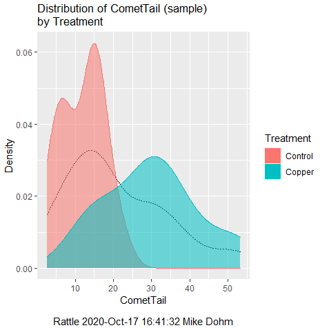
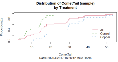
Figure 1. Rattle descriptive graphics on Comet Copper dataset. Dotted line (top image) and red line (bottom image) follow the combined observations regardless of treatment.
So, just looking at the data set, we don’t see clear evidence for a normal-like data set. The top image (Fig 1) looks stacked to the left and the cumulative plot (bottom image) is bumped in the middle, not falling on a straight line. We’ll need to investigate the assumption of normality more for this data set. We’ll begin by discussing some hypothetical points first, then return to the data set.
Goodness of fit tests of normality hypothesis
While graphics and the “eyeball test” are very helpful, you should understand that whether or not your data fits a normal distribution, that’s a testable hypothesis. The null hypothesis is that your sample distribution fits are normal distribution. In general terms, these “fit” hypotheses are viewed as “goodness of fit” tests. Often times, the test is some variation of a  problem: you have your observed (sample distribution) and you compare it to some theoretical expected value (eg, in this situation, the normal distribution). If your data fit a normal curve, then the test statistics will be close to zero.
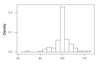
We have discussed before that the data should be from a normal distributed population. To the extent this is true, then we can trust our statistical tests are performing the way they are expected to do. We can test the assumption of normality by comparing our sample distribution against a theoretical distribution, the normal curve. I’ve shown several graphs in the past that “looked normal”. What are the alternatives for unimodal (single peak) distributions (Fig 2)?
Kurtosis describes the shape of the distribution, whether it is stacked up in the middle (leptokurtosis), or more spread out and flattened (platykurtosis).
Skewness describes differences from symmetry about the middle. Left skew the tail of the distribution extends to the left, ie, smaller values.
“Leptokurtosis”
“Platykurtosis”
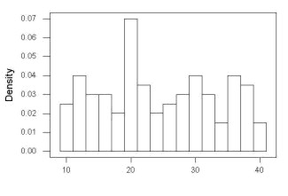
Negative skew, left skewed
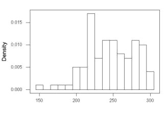
Positive skew, right skewed
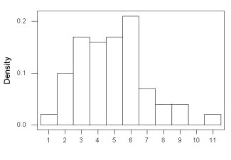
Figure 2. Graphs describing different distributions. From top to bottom: Leptokurtosis, platykurtosis, negative skew, positive skew.
The easiest procedures for goodness of fit tests of normality are based on the distribution and yield a “goodness of fit” test for normal distribution. We discussed the distribution in Chapter 6.9, and used the test in Chapter 9.1.
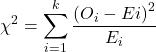
where O refers to the observed data (what we’ve got) and E refers to the expected (eg, data from a normal curve with same mean and standard deviation as our sample).
To illustrate, I simulated a data set in R.
Rcmdr: Distributions → Continuous distributions → Normal distribution → Sample from normal distribution
I created 100 values, stored them in column 1, and set the population mean = 125 and population standard deviation = 10. And therefore the population standard error of the mean was 1.0.
The resulting MIN/MAX was from 99.558 to 146.16; the sample mean was 124.59 with a sample standard deviation of 9.9164. And therefore the sample standard error of the mean was 0.9916.
Question: After completing the steps above, your data will be slightly different from mine… Why?
But getting back to the main concept, Does our data agree with a normal curve? We have discussed how to construct histograms and frequency distributions.
Let’s try six categories (why six? we discussed this when we talked about histograms).
All chi-square tests are based on categorical data, so we use the counts per category to get our data. Group the data, then count the number of OBSERVED in each group. To get the EXPECTED values, use the Z-score (normal deviate) with population mean and standard deviation as entered above.
Table 1. Tabulated values for test of normality.
| Number of observations | Weight | Normal deviate (Z) | Expected Proportion | Expected number | (Obs – Exp)2 / Exp |
| 105 | 3 | less than or equal to -2 | 0.0228 | 2.28 | 0.227368421 |
| 105 < 115 | 17 | between -1 & -2 = 0.1587 – 0.0228 | 0.1359 | 13.59 | 0.855636497 |
| 115 < 125 | 34 | between -0 & -1 = 0.5 – 0.1587 | 0.3413 | 34.13 | 0.000495166 |
| 125 < 135 | 30 | between +0 & +1 = 0.5 – 0.1587 | 0.3413 | 34.13 | 0.499762672 |
| 135 < 145 | 15 | between +1 & +2 = 0.9772 – 0.8413 | 0.1359 | 13.59 | 0.146291391 |
| > 145 | 1 | greater than or equal to +2 = 1 – 0.9772 | 0.0228 | 2.28 | 0.718596491 |
 |
Then obtain the critical value of the with df = 6 – 1 = 5 (see Appendix, Table of chi-square critical values , critical = 11.1 with df = 5).
Thus, we would not reject the null hypothesis and would proceed with the assumption that our data could have come from a normally distributed population.
This would be an OK test, but different approaches, although based on a chi-square-like goodness of fit, have been introduced and are generally preferred. We have just shown how one could use the chi-square goodness of fit approach to testing whether your data fit a normal distribution. A number of modified tests based on this procedure have been proposed; we have already introduced and used one (Wilks-Shapiro), which is easily accessed in R.
Rcmdr: Summaries → Wilks-Shapiro
Like Wilks-Shapiro, another common “goodness-of-fit” test of normality is the Anderson-Darling test. This test is now included with Rcmdr, but it’s also available in the package nortest. After the package is installed and you run the library (you should by now be able to do this!), then at the R prompt (>) type:
ad.test(dataset$variable)
replacing “dataset$variable” with the name of your data set and variable name.
In the context of goodness of fit, a perfect fit means the data are exactly distributed as a normal curve, and the test statistics would be zero. Differences away from normality increase the value of the test statistic.
How do these tests perform on data?
The histogram of our simulated normal data of 100 observations with mean = 125 and standard deviation = 10 (Fig 3).
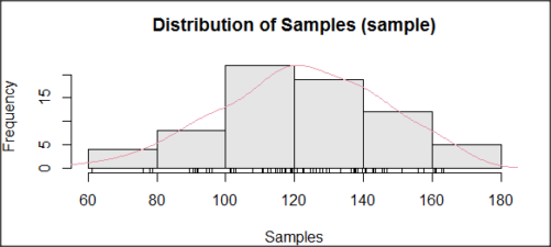
Figure 3. Histogram of simulated normal dataset, μ = 125, σ = 10.
and here’s the cumulative plot (Fig 4).
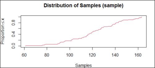
Figure 4. Cumulated frequency of simulated normal dataset, μ = 125, σ = 10.
Results from Anderson-Darling test were A = 0.2491, p-value = 0.7412, where A is the Anderson-Darling test statistic.
Results of the Shapiro-Wilks test on the same data. W = 0.9927, p-value = 0.8716, where W is the Shapiro-Wilks test statistic. We would not reject the null hypothesis in either case because p > 0.05.
Example
Histogram of a data set, highly skewed to the right. 90 observations in three groups of 30 each, with mean = 0 and standard deviation = 1 (Fig 5).
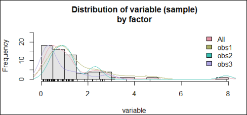
Figure 5. Histogram of simulated normal dataset, μ = 0, σ = 1.
and the cumulative frequency plot (Fig 6).
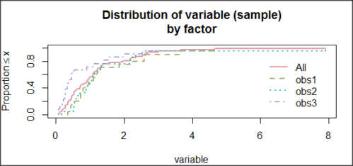
Figure 6. Cumulated frequency of simulated normal dataset, μ = 0, σ = 1.
Results from Anderson-Darling test were A = 9.0662, p-value < 2.2e-16. Results of the Shapiro-Wilks test on the same data. W = 0.6192, p-value = 6.248e-14. Therefore, we would reject the null hypothesis because p < 0.05.
The Shapiro-Wilk test in Rcmdr
Let’s go back to our data set and try tests of normality on the entire data set, ie, not by treatment groups.
Rcmdr: Statistics → Summaries → Test of normality…
normalityTest(~CometTail, test="shapiro.test", data=CometCopper)

 Shapiro-Wilk normality test

data: CometCopper$CometTail
W = 0.91662, p-value = 0.006038
End of R output
Another test, built on the basic idea of a chi-square goodness of fit is the Anderson Darling test. Some statisticians prefer this test and it is one built-in to some commercial statistical packages (eg, Minitab). To obtain the Anderson-Darling test in R, you need to install a package. After installing nortest package, run the AD test at the command prompt.
require(nortest)
ad.test(CometCopper$CometTail)

Anderson-Darling normality test

data: CometCopper$CometTail
A = 1.0833, p-value = 0.006787
End of R output.
Note 2: Because you’ve installed Rcmdr the Anderson-Darling test is available (since version 2.6) without installing the nortest package. You can call Anderson-Darling via the menu system, Statistics → Summaries → Test of normality … or type in the script the following command
normalityTest(~CometTail, test="ad.test", data=CometCopper)
In contrast, Shapiro-Wilks test is part of the base R package, so can be called directly
shapiro.test(CometCopper$CometTail)
P-values are both much less than 0.05, so we would reject the assumption of normality for this data set.
Which test of normality?
Why show you two tests for normality, the Shapiro-Wilks and Anderson-Darling? The simple answer is that both are good as general tests of normality, both are widely used in scientific papers, so just pick one and go with it as your general test of normality.
The more complicated answer is that each is designed to be sensitive to different kinds of departure from normality. By some measures, the Shapiro-Wilks test is somewhat better (ie, more statistical power to test the null hypothesis), than other tests, but this is not something you want to get into as a beginner. So, I show both of them to you so that you are at least introduced to the concept that there are often more than one way to test a hypothesis. The bottom-line is that plots may be best!
Questions
- Work describe in this chapter involves statistical tests of the assumption of normality. It is just as important, maybe more so, to also apply graphics to take advantage of our built-in pattern recognition functions. What graphic techniques, besides histogram, should be used to view the distribution of the data?
- In R, what command would you use so that you can call the variable name,
CometTail, directly instead of having to refer to the variable asCometCopper$CometTail? - Why are Anderson-Darling, Shapiro-Wilks and other related tests referred to as “goodness of fit” tests? You may wish to review discussion in Chapter 9.1.
- The example tests presented for the Comet Copper data set were conducted on the whole set, not by treatment groups. Re-run tests of normality via
Rcmdr, but this time, select the By groups option and select Treatment.
Quiz Chapter 13.3
Test assumption of normality
Data set used in this page
| Treatment | CometTail |
|---|---|
| Control | 17.86 |
| Control | 16.52 |
| Control | 14.93 |
| Control | 14.03 |
| Control | 13.33 |
| Control | 8.81 |
| Control | 14.70 |
| Control | 9.26 |
| Control | 21.78 |
| Control | 6.18 |
| Control | 9.20 |
| Control | 5.54 |
| Control | 6.72 |
| Control | 2.63 |
| Control | 7.19 |
| Control | 5.39 |
| Control | 11.29 |
| Control | 15.44 |
| Control | 17.86 |
| Contro | l4.25 |
| Copper | 53.21 |
| Copper | 38.93 |
| Copper | 18.93 |
| Copper | 30.00 |
| Copper | 28.93 |
| Copper | 15.36 |
| Copper | 17.86 |
| Copper | 17.50 |
| Copper | 21.07 |
| Copper | 29.29 |
| Copper | 28.21 |
| Copper | 16.79 |
| Copper | 21.07 |
| Copper | 37.50 |
| Copper | 38.22 |
| Copper | 17.86 |
| Copper | 29.64 |
| Copper | 11.07 |
| Copper | 35.00 |
| Copper | 49.29 |
Chapter 13 contents
- Introduction
- ANOVA Assumptions
- Why tests of assumption are important
- Test assumption of normality
- Tests for Equal Variances
- References and suggested readings
3 – Exploring data
Describing data: An introduction to summary statistics and basic visualization.
.
Scientists answer questions about natural phenomena using the scientific method. The questions in the form of hypotheses are tested by data, the raw information collected either by observing natural outcomes among groups (observational studies) or by manipulating variables (experimental studies) and recording the outcomes.
Note 1: We discussed the scientific method in Chapter 2.5. The distinction between experimental and observational studies was discussed in Chapter 2.4.
Regardless, after a study has been completed, the collection of observations needs to be summarized or described, a process now referred to as data exploration. Interpretation of the data constitutes the evidence used to evaluate the hypothesis. How many mice grew tumors in the treated versus control group? Did all mice respond to treatment? What is the typical cost of a new home in Hilo, HI? How large of a difference is there between the most expensive home and the middle? These questions require simple, summary statistics also called descriptive statistics and informative data visualizations. Both are required of any data analysis report (students: see Making a report in Mike’s Workbook for Biostatistics) — to communicate the findings of the experiment or observational study.
Note 2: Throughout Chapter 3, we present use of R Commander and R functions to accomplish our data exploration objectives. It should come as not surprise that folks have provided many solutions to improve the workflow of data exploration. rattle (R Analytic Tool To Learn Easily) is a great “data-mining” package. Rattle (version 6.5.8 as of August 2025) provides a graphical user interface, which makes it straightforward to work with. It doesn’t work well with Rcmdr, but can be used along with RStudio. rattle is an appropriate option for accomplishing tasks needed for Chapter 3, Chapter 13, and Chapter 16.
BI-311: Installing rattle is optional. Because rattle’s programming history, installation of rattle is a little different from other R packages we have described thus far. Follow instructions for your operating system at https://rattle.togaware.com/. On WinPC, download and install rattle-dev-windows-inno.exe. If you followed my R installation instructions you may need to edit the PATH environment variable on your WinPC so that R will be found by rattle. On macOS, download and extract the archived (zip) file, rattle-dev-macos.zip, and run the app (rattle.app). You will need to inform gatekeeper to allow rattle.app to run — go to Settings > Security & Privacy, and find the request to permit running the app.
In Chapter 3 we introduce two aspects of summary statistics expected in any report about a data set (see Chapter 4 — How to report statistics). Summary statistics provide a brief overview of relevant characteristics of observations in the data set to provide the reader to get a quick but meaningful look at the data set. Data set refers to a collection of data, usually a collection of related, ordered observations, measurements, and related information.
Summary statistics vary according to the needs of the reporting vehicle, but may generally address two characteristics of the data set
- Central tendency or the description of the middle of the data. See Chapter 3.2 – Measures of Central Tendency.
- Data dispersion, the variability around the middle of the data set. See Chapter 3.3 – Measures of dispersion.
- The other two sections in Chapter 3 introduce estimation, the role random sampling plays, and the kinds of error in statistics (Chapter 3.4 — Estimating parameters).
- The final section, 3.5 – Statistics of error, introduces incorporating estimates of error in measurement calculations are used to report confidence — confidence intervals — in the estimates we make.
Before we can talk about descriptive statistics we need to introduce the concept of data types, which we do in Chapter 3.1 — Data types. Understanding data types is crucial for accurately calculating and interpreting measures of central tendency and dispersion, which are essential for effective data visualization.
We introduce statistical graphics, a specialized kind of data visualization, in Chapter 4 – How to report statistics . Statistical graphs are utilized to describe data sets, but also to communicate statistical inference, which we address formally beginning in Chapter 7 – Probability, Risk Analysis.
Formulas — a reminder.
Most of you have been asked at some point to calculate the average or the sample standard deviation. We will provide these again, but with additional statistics. Textbooks may present calculator formulas — nothing wrong with them, although we have to watch significant figures. But computer statistical packages generally do not use these formulations as the approach to calculate — the algorithms are typically much more involved. So why present formulas throughout the book as I do? Formulas often are the best definition of the statistical concept. I haven’t investigated this last point in any systematic way, but, because of access by scientists to increasingly powerful computers since the 1980s, I doubt anyone in the business of data analysis in the biological sciences has much use of the hand calculator or the formulas except as definitions.
Note 3. Chaminade University students: On homework, quizzes and exams, you may be asked to calculate these descriptive statistics. The data sets will always be simple ones, simple enough that calculators should not be needed.
Homework to go with this topic.
Mike’s Workbook for Biostatistics:
Homework 2A: Descriptive statistics
Quizzes in this chapter
A total of 56 questions among the several subchapters, a mix of true or false and multiple choice question format.
Chapter 3 contents
.