6.3 – Combinations and permutations
Introduction
In statistical inference, an important foundational skill is to be able to count the possible outcomes of an experiment — the sample space. For example, when drawing on a sample of individuals for study from specific groups (strata) of a population, combinations may be calculated; where it is unwarranted to assume a particular theoretical probability distribution applies, permutation tests create a reference distribution by calculating all possible values of a test statistic under rearrangements of the observed data.
The simplest place to begin with probability is to define an event — an event is an outcome — a “Heads” from a toss of coin, or the chance that the next card dealt is an ace in a game of Blackjack. In these simple cases we can enumerate how likely these events are given a number of chances or trials. For example, if the coin is tossed once, then the coin will either land “Heads” or “Tails” (Fig 1).
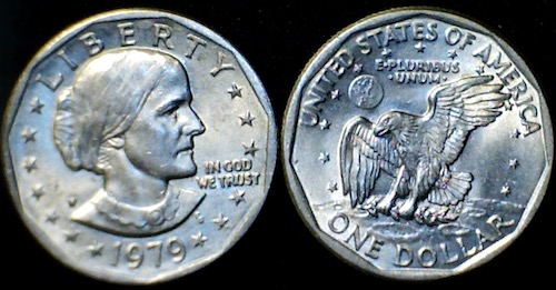
Figure 1. Heads (left) and Tails (right) of a USA Susan B. Anthony dollar.
We can then ask what is the likelihood of ten “Heads” in ten tosses of a fair coin?
And this gets us to some basic rules of probability:
- if successive events are independent, then we multiply the probability
- if events are not independent, then the probability adds
- do we sample without replacement, ie, an object can only be used once?
- do we sample with replacement, ie, an object gets placed “back in the deck” and can be used again and again
Combinations and Permutations
Both combinations and permutations pertain to how samples are selected from a population. Combinations are used if the events or objects of the sample are all of the same kind, whereas for permutations, it is implied that the events or objects are not all of the same kind.
Figure 2. A combination lock
Combinations ignore the order of the events; permutations are ordered combinations. For replacement, the formula for permutations is simply 
In the case of the ten “Heads,” in ten successive trials, the probability is  “ten-times” or
 = 0.0009766 (in R, just type
0.5^10 or (1/2)^10 at the R prompt).
Examples of permutations in biology include,
Given the four nucleotide bases of DNA, adenine (A), cytosine (C), guanine (G), and thymine (T), how many codons are possible?

where the three (3) refers to the codon, three nucleotide genetic code. Codons are trinucleotide sequences of DNA or RNA that correspond to a specific amino acid. For transcription initiation of a protein-coding gene, a key sequence must be present in the promoter region of the gene. In Archaea and Eukaryotes, that sequence is called the TATA box. How often do we expect to find by chance the heptamer (ie, seven bases) TATA box sequence in the human genome?
Note 1: The consensus TATA box sequence, TATAWAW (W can be either Adenine or Thymine, per Standard IUB/IUPAC nucleic acid code). The TATA box is the binding site for transcription factors, particularly the TATA binding protein.

Thus, we would expect at random to find TATA box sequences every 16,384 bases along the genome. For the human genome of 3.3 billion bases then we would expect at random more than 200,000 TATA box consensus sequences.
Another way to put this is to ask how many combinations of ten tosses gets us ten “Heads” then weigh this against all possible outcomes of tossing a coin ten times — how many times do we get zero Heads? Two “Heads”? And so on. This introduces the combinatorial.
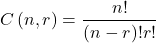
where n is the number of choices (the list of events) and r is how many times you choose or trials. The exclamation point is called the factorial. The factorial instructs you to multiply the number over and over again, “down to one.” For example, if the number is 10, then

In R, just type factorial(10) at the R prompt.
factorial(10)
[1] 3628800
An example
Consider an extrasensory perception, ESP, experiment. We place photocopies of two kinds of cards, “Queen” and “King,” into ten envelopes, one card per envelope (Fig 2). Thus, an envelope either contains a “Queen” or a “King.”

Figure 2. Playing cards with images commemorating 150th anniversary of Charles Darwin’s Origin of Species. (Design John R. C. White, Master of the Worshipful Company of Makers of Playing Cards 2008 to 2009.)
We shuffle the envelopes containing the cards and volunteers guess the contents of the envelopes, one at a time. We score the correct choices after all envelopes had been guessed. (It’s really hard to set these kinds of experiments up to rule out subtle cues and other kinds of experimental error! Diaconis 1978, Pigliucci 2010, pp. 77 – 83.) By chance alone we would expect 50% correct (eg, one way to game the system would have been for the volunteer simply to guess “Queen” every time; since we had placed five “Queen” cards the volunteer would end up being right 50%).
What are the possible combinations?
Let’s start with one correct; the volunteer could be right by guessing the first one correctly, then getting the next nine wrong, or equivalently, the first choice was wrong, but the second was correct followed by eight incorrect choices, and so on.
We need math!
Let n = 10 and r = 1
Using the formula above we have
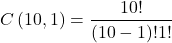
or ten ways to get one out of ten correct. This is the number of combinations without replacement.
In R, we can use the function choose(), included in the base install of R. At the R prompt type
choose(10,1)
and R returns
[1] 10
For permutations, use choose(n,k)*factorial(k).
To get permutations for larger sets, you’ll need to write a function or take advantage of functions written by others and available in packages for R. See gtools package, which contains programming tools for R. There are several packages that can be used to expand capabilities of working with permutations and combinations. For example, install a package and library called combinat and then run the combn() function, together with the dim() function, which will return
dim(combn(10,1))[2]
[1] 10
R explained
In the combn() the “10” is the total number of envelopes and the “1” is how many correct guesses. We also used the dim() function to give us the size of the result. The dim() function returns two numbers, the number of rows and the number of columns — combn() returns a matrix and so dim() saves you the trouble of counting the outcomes — the “[2]” tells R to return the total number of columns in the matrix created by combn(). Here’s the output from combn() , but without the dim() function
combn(10,1)
     [,1] [,2] [,3] [,4] [,5] [,6] [,7] [,8] [,9] [,10]
[1,]    1    2    3    4    5    6    7    8    9    10
in order, we see that there is one case where the success came the first time [1,1], another case where success came on the second try [1,2] and so on.
We can write a simple function to return the combinations
for (many in seq(0, 10, by = 1)){
    print(choose(10, many))
}
an inelegant function, but it works well enough, returning
[1] 1
[1] 10
[1] 45
[1] 120
[1] 210
[1] 252
[1] 210
[1] 120
[1] 45
[1] 10
[1] 1
Note that there’s only one way to get zero correct, only one way to get all ten correct.
For completion, what would be the permutations? Use the permn() function (same combinat library) along with length() function to get the number of permutations
length(permn(10))
[1] 3628800
Continue the example
Back to our ESP problem. If we continue with the formula, how many ways to get two correct? Three correct? And so on, we can show the results in a bar graph (Fig 3).
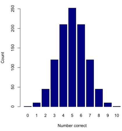
Figure 3. Bar chart of the combinations of correct guesses out of 10 attempts (graph was presented in Chapter 4.1).
The graph in Figure 3 was made in R
Combos <- seq(0,10, by=1)
HowMany <- c(1,10,45,120,210,252,210,120,45,10,1)
barplot(HowMany, names.arg = Combos, xlab = "Number correct", ylab = "Count",col = "darkblue")
If you recall, we had two students score eight out of ten. Is this evidence of “ESP?” It certainly seems pretty good, but how rare is this to score 8 out of 10? The total number of outcomes was

Eight out of ten could be achieved in 45 different ways, so
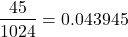
So, eight out of ten is pretty unlikely! Is it evidence for ESP powers in our Biostatistics class? In fact, at the traditional Type I error rate of 5% used in biology and other sciences to evaluate inferences from statistical tests (See Chapter 8), we would say that this observation was statistically significant. Given that this would be an extraordinary claim, this should give you an important clue that statistical significance is not the same thing as evidence for the claim of ESP.
Note 2: This is a good example where frequentist approach may not be the best approach — the Bayesian prior probability for ESP is vanishingly low. See O’Hagan (2006) for a similar ESP problem worked from a Bayesian perspective.
In other words, Is our result biologically significant? Probably not, but I’ll keep my eyes on you, just in case.
Conclusions
Combinations or permutations?
Combinations refers to groups of n things taken k times without repetition. Note that order does not matter, just the combination of things. Permutations, on the other hand, specifically relate the number of ways a particular arrangement can show up.
Questions
- Calculate the combinations, from zero correct to ten correct, from our ESP experiment, ie, confirm the numbers reported in Figure 3.
- Consider our ESP tests based on guessing cards. Let’s say that one subject repeatedly reports correct guesses at a rate greater than expected by chance. Why or why not should we view this as evidence the person may have extrasensory perception?
- Return to our TATA box example. The number of protein-coding genes in the human genome is presently estimated to be 20,620 (NCBI August 2025). Given that each gene has one promoter sequence, what proportion of TATA boxes are not associated with protein-coding genes?
- Assuming a standard 52-card deck, how many possible 5-card poker hands — the set of cards a player holds during a round of play — are there?
Quiz Chapter 6.3
Combinations and permutations
Chapter 6 contents
- Introduction
- Some preliminaries
- Ratios and probabilities
- Combinations and permutations
- Types of probability
- Discrete probability distributions
- Continuous distributions
- Normal distribution and the normal deviate (Z)
- Moments
- Chi-square distribution
- t distribution
- F distribution
- References and suggested readings
6.1 – Some preliminaries
Introduction
OK, you say, I get it: statistics is important, and if I am to go on as a biologist, I should learn statistics. Let’s get on with it, start with the equations and the problems already!
Before we review probability theory and introduce risk analysis I want to spend some time to emphasize that at issue is critical thinking, so please bear with me (Fig 1).
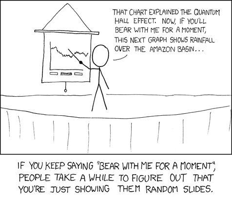
Figure 1. “Slides,” https://xkcd.com/365/.
How likely?
As we start our journey in earnest, we start with the foundations of statistics, probability. Probability in statistics means the chance that a specific outcome will occur. Probability is something we measure, or estimate, or draw from theoretical models, about whether something, a specific outcome from a class of outcomes (events — see Chapter 7.1), will occur. We speak about how likely an outcome is to occur, and this is quantified by the probability. Probabilities are given a value between 0 and 1: at 0% chance, the event will not happen; 100% chance, the event is certain to happen. Remember, probability applies to predicting future events; obviously, when viewed in the past, the event either did (100%), or did not (0%) happen.
If probability is the chance that an outcome will occur, then risk is the probability of a particular outcome occurring over a specified period of time. Related, epidemiologists define exposure risk as the potential for harm (or benefit) from contact with or vulnerability to a hazard (or treatment) or risk factor.
I introduce our discussion of probability through a risk analysis — the process of evaluating the probability and potential impact of health risks to individuals or populations. I like to start this discussion by relaying something I overheard while a number of us were standing on a lava field on the slopes of Kilauea back in November of 1998 (Kilauea erupted with lava flow more or less continually between 1983 and 2018; 5 Jan 2023, started up again).

Figure 2. View of Kamokuna Lava Bench, eruption of Pu`u `O`o, Kilauea, November 1998. Photo by S. Dohm.
In 1998, Volcanoes National Park hadn’t established barricades at the end of Chain of Craters Road, and people were walking to see new lava flows. The night we went, we met a park ranger who pleaded with us that the Park Service believed it was unsafe for us to walk out to see new lava flows because the area, called a lava delta, was unstable. Someone (not in my group), snapped back, “Oh, what are the chances that that will happen?” Of course, the ranger couldn’t quote a chance between zero and 100% for that particular evening. The ranger was saying the risk had increased, based on their subjective, but experienced opinion (see Kinds of probability, below).
As you can see in Figure 2, we went anyway. I have been thinking about her question ever since. We were lucky — some of the same area collapsed two weeks later (SOEST information, eruption about episode 55).
Cool picture though.
While the terms are used interchangeably in everyday language, they have distinct mathematical and statistical definitions. Prospective: You use a known model and its parameters to predict the probability of future data.
Multiple events
Whether or not a newly formed lava delta collapses, that’s a singular or simple event. For cases with more than one one outcome, that’s a multiple event.
I have two coins, a dime and a quarter, in my pocket; when I place the coins on the table, what are the chances that both coins will show heads? A blood sample from a crime scene was typed for two Combined DNA Index System (CODIS) Short Tandem Repeat (STR) loci, THO1 (allele 9.3) and TPOX (allele 8), the same allele types for the defendant. What are the chances of a match, someone other than the defendant has the same genetic profile? In both examples I describe a random process. With randomness, we can predict the probability of each kind of outcome, or series of outcomes, because we know the total possible number of outcomes. If there are just two outcomes, then the probability is equal — 50% that either will occur. If, however, the process is not random, then even if there are just two possible outcomes, the probability can’t be 50% — the outcome depends on some other process than random chance.
What is the chance that two events occur? For two or more independent events we can get the answers by using the product rule.

The two coins are independent, therefore the chance that both are placed heads up is 25% — we would expect to see this combined event one out of every four times. This is an illustration of the counting rule, aka fundamental counting principle: if there are n ways to do one thing (n elements in set A), and m ways to do another thing (m elements in set B), then there are  ways to do both things (combination of elements of A and B sets).
For the DNA profile CODIS problem (cf. Chapter 4, National Research Council 1996), the two alleles are both the most common observed in US Caucasian population at 30.45% and 54.7%, respectively (Moretti et al 2016). Assuming the individual was homozygous at both loci (ie, THO19.3,9.3 and TPOX8,8), then the genotype frequencies (p2) are:


Since THO1 is located on the p arm of chromosome 11, and TPOX is on the p arm of chromosome 2, the two loci are independent and therefore should be in linkage disequilibrium. We can use the product rule to get the probability of the DNA profile for the sample, 2.8%

If two events are not independent, then the product rule cannot be used. For example, CODIS STR D5S818 and CSF1PO are both located on the q arm of chromosome 5 and are therefore linked and not independent (the recombination frequency is about 0.25). The common allele for D5S818 is 11 at 40.84% and for CSF1PO the allele is 12 at 34.16%. Thus the chance that the two most common alleles is not simply the product rule result of 14%, instead we need to view this problem as one of dependent events.
Kinds of probability.
So, how does one go about estimating the likelihood that a particular event, whether it is collapse of a lava delta, or that a person will have a heart attack? The probability of lava delta collapse or of heart attack are examples of empirical probability, as opposed to a theoretical probability. Despite many years of effort, we have no applicable theory that we can apply to say, if a person does this, and that, then a heart attack will happen. But we do have a body of work documenting how often heart attacks occur, and when they occur in association with certain risk factors. Similarly, progress is being made to determine markers of risk of lava field collapse (Di Traglia et al. 2018). Analogously, this is the essential goal of risk analysis in epidemiology. We know of associations between cholesterol and heart attack risk, for example, but we also know that high cholesterol does not raise the probability of the event (heart attack) to 100%. How is this uncertainty part of statistics? Or perhaps you are a molecular scientist in training and have learned about how to assess results of a Western blot where typically the results are scored as “yes” or “no.” How is this relevant to statistics and probability?
A misconception about statistics and statistical thinking
There’s a long history of skepticism of conclusions from health studies, in part because it seems the advice flips. For example,
- Coffee is bad for you (Medical News Today January 2008)
- Coffee is good for you (NBC News July 2018)
- Even light drinking can be harmful to health (Science Daily, January 2022)
- Seven science-backed reasons beer is good for you (NBC News August 2017)
- Meat and cheese may be as bad for you as smoking (Science Daily, March 2014)
- Cheese actually isn’t bad for you (WIRED, February 2021)
The common thread is these studies are assessment of risk: about studies that seem to conclude “only: with statements of probability.
Perhaps you may have heard …? “There are lies and then there is statistics“. The full quote reads as follows:
Figures often beguile me, particularly when I have the arranging of them myself; in which case the remark attributed to Disraeli would often apply with justice and force: “There are three kinds of lies: lies, damned lies and statistics.” – Autobiography of Mark Twain (www.twainquotes.com/Lies.html).
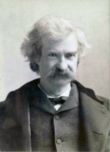
Figure 3. Mark Twain. Image from The Miriam and Ira D. Wallach Division of Art, Prints and Photographs: Photography Collection, The New York Public Library. “Mark Twain in Middle Life” The New York Public Library Digital Collections. 1860 – 1920. https://digitalcollections.nypl.org/items/510d47d9-baec-a3d9-e040-e00a18064a99
Twain attributed the remarks to Benjamin Disraeli, the prime minister of Britain during much of Queen Victoria’s reign, but others have not been able to document this utterance to that effect. Still others believe that the “3-lies” quote belongs to Leonard Courtney, an English mathematician and statistician (1847-1929) (see University of York web site for more).
What is meant by this quote? Tossing aside cynicism — or healthy skepticism of authority one should have, whether that authority is a scientist or a politician(within reason, please!) — what this quote means is that it seems that results of very similar studies are in conflict. To some, this is part of the replication crisis in science (Baker 2016). There’s a perception that one can say just about anything with a number. Partly this is a matter of semantics, but also there is legitimacy to this concern. However, it is not necessarily the case that statistics have been intentionally done to mislead, rather, there is evidence that researchers are not always using proper statistical procedures.
One word, several meanings
We use the term statistics in multiple ways, all correct, but not all equal. For example, a statistic may refer to a number used to describe a population characteristic. From the 2010 U.S. census, we learn that the racial (self-reported) make-up of the U.S. population (then at 303 million) was 72.4% “white” and 12.6% “black” self-reported. In this sense, a statistic is something you calculate as a description. Do you recall the distinction between “statistic” and “statistics” discussed in Chapter 2?
Secondly, two studies essentially about the same topic, yet reaching seemingly different conclusions, may differ in the assumptions employed. It should be obvious that if different assumptions are used, researchers may reach different outcomes.
Finally, how we communicate statistics can be misleading. For example, use of percentages in particular can be confusing, especially in communication of the chance that some event may happen to us (eg, incidence of disease: number of new cases in a specific time period, compared to prevalence of a disease: number of cases of a disease in a specific period of time). On the one hand, percentages seem easy. A percentage is simply a proportion multiplied by 100%, and takes any value between 0% and 100%.
When a product says that it kills 99.99% of all germs on contact, do you feel better? Here’s a cartoon to consider as you think about that statement (Fig 4).
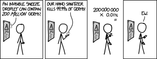
Figure 4. “Hand sanitizer,” https://imgs.xkcd.com/comics/hand_sanitizer.png
Of course numbers cannot be used to justify simultaneously mutually exclusive conclusions, but being able to recognize careless (or deliberate) miscommunication with numbers, well, this needs to be part of your skill set. Here’s a little exercise from transportation safety to ponder as you reflect on the subject of lies and statistics. rather, as you read this next section I ask that you consider
- are the correct statistical descriptors in use?
- what assumptions are being made?
- does the reporting of percentages lead to clear conclusions?
Some concluding thoughts about “lies and statistics”
Statistics is tricky because there are assumptions to be made. And you have to be clear in your thinking.
If the assumptions hold true, then we aren’t lying, and Twain had it wrong.
But if we disagree on the assumptions, then we will necessarily have to disagree on the conclusions drawn from the calculated numbers (the statistics). Risk analysis in particular, but statistics in general, is a tricky business because many assumptions need to be made, and we won’t necessarily have all of the relevant information available to make sure our assumptions are truthful. But it is the assumptions that matter: if we agree with the assumptions that are made, then we have confidence in the conclusions drawn from the statistics.
In a typical statistics course, we would spend a bunch of time on probability. We will here as well, but in the context of risk analysis and in the other contexts, in a less than formal presentation on the subject of probability. For example, in talking about inference, the testing of null hypotheses and estimating the probability that the null hypothesis is correct, I will say things like, “Imagine we repeated the experiment a million times — how many times by chance would we think a correct null hypothesis would none the less be rejected?”
There’s no real substitute for a formal course in probability theory and you should be aware that this foundation is pretty important if you go forward with biostatistics and epidemiology. For now, I will simply refer you to chapters 1, 2 and 3 of a really nice online book on probability from one of the masters, Richard Jeffrey (1926 – 2002; click here to go to Wikipedia). Much of what I will present to you follows from similar discussions.
My aim is to teach you what you need about probability theory by the doing. In the next couple of days we will deal with an aspect of risk analysis, namely a consideration of conditional probability and Baye’s Theorem that will help you evaluate claims such as the one made for airline safety. Risk analysis is tricky, but it is not a subject above and beyond our abilities; by applying some of the rules of statistical reasoning, we can check claims based on statistics. A healthy degree of skepticism is part of becoming a scientist. Do try this at home!
Some examples to consider: what is the relative risk for the following scenarios?
1. Drug testing at the workplace: risk of a worker, who does not use illegal drugs, registering positive (false positives in drug testing);
2. Positive HIV from blood sample from USA male with no associated risks (eg, intravenous drug user), false positives in HIV testing; false positives with mammography;
3. Benefits versus risks of taking a statin drug (drug that reduces serum cholesterol levels) to a person with no history of heart disease.
4. Is it safer to travel by car or by airliner? We’ll break this problem down in the next section.
What we are looking for is the probability of an occurrence of a particular event: that a person who does not use illegal drugs may nonetheless test positive; we are looking for a way to make rational decisions and understanding probability is the foundation.
Questions
- What do you make of the claim (joke) that “There are lies and then there are statistics?”
- Distinguish between empirical and theoretical probability; use examples.
Quiz Chapter 6.1
Some preliminaries
Chapter 6 contents
- Introduction
- Some preliminaries
- Ratios and proportions
- Combinations and permutations
- Types of probability
- Discrete probability distributions
- Continuous distributions
- Normal distribution and the normal deviate (Z)
- Moments
- Chi-square distribution
- t distribution
- F distribution
- References and suggested readings
5.6 – Sampling from Populations
Introduction
Researchers generally can’t study an entire population. More generally, striving to study each member of a population is not necessary to arrive at answers about the population. For example, consider the question, does taking a multivitamin daily improve health? What are our options? Do we really need to follow every single individual in the United States of America, monitoring their health and noting whether or not the person takes vitamins daily in order to test (inference) this hypothesis? Or, can we get at the same answer by careful experimental design (see Schatzkin et al 2002; Dawsey et al 2014)? Supplement use is wide-spread in the United States, but both health and vitamin use differ by demographics. Young people tend to be healthier than older people and older people tend to take supplements more than younger people.
A subset of the population is measured for some trait or characteristic. From the sample, we hope to refer back to the population. We want to move from anecdote (case histories) to possible generalizations of use to the reference population (all patients with these symptoms). How we sample from the reference population limits our ability to generalize. We need a representative sample: simple to define, hard to achieve.
Statistics becomes necessary if we want to infer something about the entire populations. (Which is usually the point of doing a study!!) Typically tens to thousands of individuals are measured. But in addition, HOW we obtain the sample of individuals from the reference population is CRITICAL.
Kinds of sampling include (adapted from Box 1, Tyrer and Heyman 2016; see also McGarvey et al 2016)
Probability sampling
- random
- stratified
- blocking
- clustered
- systematic
Nonprobability sampling
- convenience, haphazard
- judgement
- quota
- snowball
For an exhaustive, authoritative look at sampling, see Thompson (2012).
How can samples be obtained?
Sampling from a population may be convenient. For one famous example, consider the Bumpus data set. (We introduced this data set in Question 5, Chapter 5.) So the legend goes, Professor Bumpus was walking across the campus of Brown University, the day after a severe winter storm, and came across a number of motionless house sparrows on the ground. Bumpus collected the birds and brought them to his lab. Seventy-two birds recovered; 64 did not (Table1).
Table 1. A subset of Bumpus data set, summarized by sex of birds.
| House sparrows | Lived | Died |
|---|---|---|
| Female | 21 | 28 |
| Male | 51 | 36 |
Bumpus reported differences in body size that correlated with survival (Bumpus 1899), and this report is often taken as an example of Natural Selection (cf. Johnston et al 1972). The Bumpus dataset is clearly convenience sampling. It’s also a case study: a report of a single incident. But given that is is a large sample (n = 136), it is tempting to use the data to inform about about possible characteristics of the birds that survived compared with those that perished.
Another way we collect samples from populations is best termed haphazard. In graduate school I got the opportunity to study locomotor performance of whiptail lizards (Aspidoscelis tigris, A. marmoratus, genus formerly Cnemidophorus**) across a hybrid zone in the Southwest United States (Dohm et al. 1998). During the day we would walk in areas where the lizards were known to occur and capture any individual we saw by hand. (This would sometimes mean sticking our hands down into burrows, which was always exciting — you never really knew if you were going to find your lizard or if you were going to find a scorpion, venomous spider, or …) Lizards collected were returned to the lab for subsequent measures. Clearly, this was not convenience sampling; it involved a lot of work under the hot sun. But just as clearly, we could only catch what we could see and even the best of us would occasionally lose a lizard that had been spotted. Moreover, one suspects we missed many lizards that were present, but not in our view. Lizards that were underground at the time we visited a spot would not be seen nor captured by us; individual lizards that were especially wary of people (Bulova 1994) would also escape us. In other words, we caught the lizards that were catchable and can only assume (hope?) that they were representative of all of these lizards. Applying a grid or quadrant system to the area and then randomly visiting plots within the grid or quadrant might help, but still would not eliminate the potential for biased sampling we faced in this study.
Quota sampling implies selection of subjects by some specific criteria, weighted by the proportions represented in the population. It’s different from stratified sampling because there is no random selection scheme: subjects are selected based on matching some criteria, and collection for that group stops when the sample number matches the proportion in the population. Consider our vitamin supplement survey. If student population at Chaminade University was the reference population, and we have enough money to survey 100 students, then we would want a sample of 70 women students and 30 male students, representing the proportions of the student population.
Snowball sampling implies that you rely on word-of-mouth to complete sampling. After initial recruitment of subjects, sample size for the study increases because early participants refer others to the researchers. This can be a powerful tool for reaching underrepresented communities (eg, Valerio et al 2016).
Types of Probability sampling
Random sampling is an example of probability sampling. As we defined earlier, simple random sampling requires that you know how many subjects are in the population (N) and then each subject has an equal chance of being selected

Examples of nonprobability sampling include
- convenience sampling
- volunteer sampling
- judgement sampling
Convenience sampling (the first 20 people you meet at the library lanai); volunteer sampling (you stand in front of a room of strangers and ask for any ten people to come forward and take your survey — or more seriously, persons with a terminal disease calling a clinic reportedly known to cure the disease with a radical new, experimental treatment), and judgement sampling (to study tastes in fashion, you decide that only persons over six feet tall should be included because .…).
Random in statistics has a very important, strict meaning. As opposed to our day-to-day usage, random sampling from a population means that the probability that any one individual is chosen to be included in a sample is equal. Formally, this is called simple random sampling to distinguish it from more complex schemes. For a sampling procedure to be random requires a formal procedure for sampling a population with known size (N).
For example, at the end of the semester, I may select the order for student presentations at random. Thus, students in the classroom would be considered the population (groups of students are my sample unit, not individual students!). What is the probability that your group will be called first? Second? We need to know how many groups there are to conduct simple random sampling. Let’s take an extreme and say that all groups have a size of one; there are 26 students in this room, so

or

of being selected first.
Now to determine the probability of your group being selected second, we need to distinguish between two kinds of sampling:
- Sampling with replacement — after I select the first group, the first group is returned to the pool of groups that have not been selected. In other words, with replacement, your group could be selected first and selected second! The probability of being selected second then remains

.
- Sampling without replacement — after I select the first group, then I have

groups left to select the second group, so probability that your group will be second is

. The first group has already been selected and is not available.
Random sampling refers to how subjects are selected from the target, reference population. Random assignment, however, describes the process by which subjects are assigned to treatment groups of an experiment. Random sampling applies to the external validity of the experiment: to the extent that a truly random sample was drawn, then results may be generalized to the study population. Random assignment of subjects to treatment however makes the experiment internally valid: results from the experiment may be interpreted in terms of causality.
R code, sample without replacement
sample(26)
[1] 1 10 11 23 17 13 8 6 19 20 21 16 14 15 5 2 12 4 26 22 9 7 25 18 3 24
R code, sample with replacement
mySample <- sample(26, replace = TRUE); mySample
[1] 9 26 24 9 3 1 23 14 26 6 5 19 17 23 11 12 3 8 7 19 2 16 3 11 1 1
How many elements duplicated?
out <- duplicated(mySample); table(out)
out
FALSE TRUE
17 9
More on sampling in R discussed in Sampling with computers below.
Additional sampling schemes
Simple random sampling is not the only option, but in many cases it is the most desirable. Consider our multivitamin study again. Perhaps studying the entire USA population is a bit extreme. How about working from a list of AARP members, sending out questionnaires to millions of persons on this list, getting back about 20% of the questionnaires, sorting through the responses and identifying the respondent to diet categories and multivitamin use. The researchers had nearly 500,000 persons willing and able to participate in their prospective study (Schatzkin et al 2001; Dawsey et al 2014; Lim et al 2021). It’s an enormous study. But is this really much better than our described lizard experiment? Let’s count the ways: Not all older people are members of AARP (that 500,000? That’s less than 1% of the 50 and older persons in the USA); A large majority of AARP members did not return surveys; Some fraction of the returned surveys were not usable; How representative of diverse aged populations in the United States is AARP?
Simple random sampling may not be practical, particularly if sub-populations, or strata, are present and members of the different sub-populations are not available to the researcher in the same numbers. In ecology, habitat-use studies routinely need to account for the patchiness of the environment in space and time (Wiens 1976; Summerville and Crisp 2021). Thus, samples are drawn in such a way to represent the frequency within each sub-population.
For a simple example, researchers conducting a controlled breeding program of mice don’t use simple random sampling to choose pairs of mates; after all, random sampling without regard of sex of the mice would lead to some pairings of males only, or females only (Fig 1).
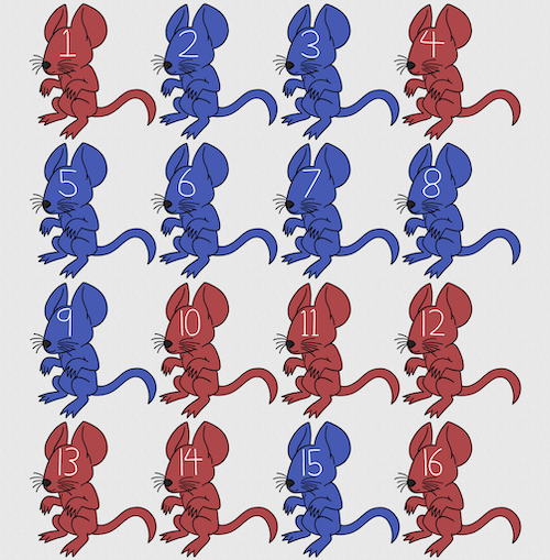
Figure 1. Sixteen mice, eight red and eight blue. Image © 2024 Mia D Graphics
R code
pairs <- c(rep("red", 8), rep("blue", 8))
replicate(2, sample(pairs, 8), simplify = FALSE)
[[1]]
[1] "blue" "blue" "blue" "red" "blue" "red" "blue" "red"

[[2]]
[1] "blue" "blue" "red" "red" "red" "red" "red" "blue"
Oops. If we interpret the output blue = male and red = female, then four out of the eight pairs were same sex pairings.
Thus, the breeding strategy is to random sample from female mice and from male mice and the stratification is sex of the mouse. Alternatively, breeders may select mice to form breeding pairs systematically: From a large colony with dozens of cages, the breeder may select one mouse from every third cage.
Stratified Random Sampling: Individuals in the population are classified into strata or sub-groups: age, economic class, ethnicity, gender, sex …, as many as needed. Then choose a simple random sample from each group, typically in proportion to the size of the sub-groups in the population. Combine those into the overall sample. For example, when I wanted a random sample of mice for my work, I called the supplier and requested that a total of 100 male and female mice be randomly selected from the five colonies they maintained. The reference population is the entire supply of mice at that company (at that time), but I wished to make sure that I got unrelated mice, so I needed to divide the population into groups (the five colonies) before my sample was constructed.
Note 1: The size of the population must be known in advance, just like in simplified random sampling. A more interesting example, the Social Security Administration conducts surveys of popular baby names by year. They post the top ten most popular names based on 1% or 5% (first strata), then by male/female (second strata).
For a simple example of the need for stratified sampling, consider our 16 blue and red mice again. If mice were randomly assigned to treatment group, then by chance unequal samples within strata may be assigned to a treatment group, potentially biasing our conclusions (Fig 2).
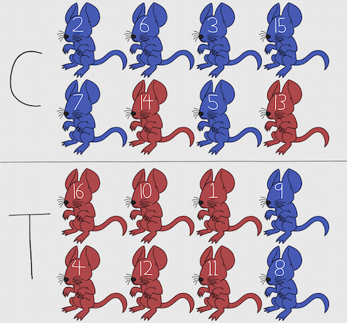
Figure 2. Sixteen mice, randomly assigned to treatment groups C and T; by chance, 75% blue in C and just 25% in T. If color was a confounding factor then our conclusions about the effectiveness of the treatment would be associated with color. Image © 2024 Mia D Graphics
Block sampling: superficially resembles stratified sampling, but refers to how experimental units are assigned to treatment groups. Blocks in experimental design refers to potentially confounding factors for which we wish to control, but are otherwise not interested in. For our example described in Figure 2, mouse color may not be of specific interest for our study and therefore would be considered a blocking effect.
Agricultural research provides a host of other blocking situations: plots distributed across an elevation or hydration gradient (Fig 3), soil types, and many others.

Figure 3. Agricultural fields in Central Poland. NASA https://visibleearth.nasa.gov/images/146593/agriculture-fields-in-central-poland/146595w
For a microbiology example, edge effects of heated culture plates. For a growth experiment it’s unlikely we are specifically interested in the plate layout on the growth characteristics of treated cells. However, it’s also unlikely we can assume placement has no influence on growth (eg, Mansoury et al 2021). A 96-well microplate has 60 inner wells and 36 edge wells (A1 – H1, A12-H12, plus 1st and 12th wells of columns B – H, for a total of 36 wells, Fig 4). Thus, analysis of growth effects should include a block effect for well position.
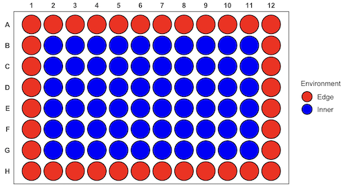
Figure 4. Format of 96-well plate. Red cells = “edge” wells; blue cells = “inner” wells. Plotted with ggplate package.
For long incubation periods it’s not unexpected that edge wells and inner wells may evaporate at different rates, potentially confounding interpretation of treatment effects if, by chance, treatment samples are more commonly assigned to edge wells. Block sampling implies subjects from treatment groups are randomly assigned to each block, in equal numbers if possible.
Cluster Sampling: In many situations, the population is far too large or too dispersed and scattered for a list of the entire population to be known. And, a random approach ignores that there is a natural grouping — people live next to each other, so there is going to be things in common. A multi-stage approach to sampling will be better than simply taking a random sample approach. Most surveys of opinion (when conducted reputably) use a multi-stage method. For example, if a senator wishes to poll his constituents about an issue, he may his pollster will randomly select a few of the counties from his state (first stage), then randomly select among towns or cities (second stage), to obtain a list of 1000 people to call. In some instances, they might use even more stages. At each stage, they might do a stratified random sample on sex, race, income level, or any other useful variable on which they could get information before sampling. If you are interested in this kind of work, for starters, see Couper and Miller (2009).
There are more types of sampling, and entire books written about the best way to conduct sampling. One important thing to keep in mind is that as long as the sample is large relative to the size of the population, each of the above methods generally will get the same answers (= the statistics generated from the samples will be representative of the population).
As long as some attempt is made to randomize, then you can say that the procedure is probability sampling. Nonprobability, or haphazard sampling, describes the other possibility, that is, each element is selected arbitrarily by a non-formal selecting of individual. … all the fish or birds that you catch may not be a random sample of those present in a population. For example,
- wild Pacific salmon do not feed on the surface, hatchery salmon feed on the surface. …
- all the individuals who respond to a survey.
- Phone surveys, web surveys, person on the street surveys… how random, how representative?
Sampling with computers
Now to determine the probability of your group being selected second, we need to distinguish between two kinds of sampling:
Sampling with replacement — after I select the first group, the first group is returned to the pool of groups that have not been selected. In other words, with replacement, your group could be selected first and selected second! The probability of being selected second then remains
Sampling without replacement — after I select the first group, then I have

groups left to select the second group, so probability that your group will be second is

. The first group has already been selected and is not available, and so on.
Sampling is usually easiest if a computer is used. Computers use algorithms to generate pseudo-random numbers. We call the resulting numbers pseudo-random to distinguish them from truly random physical processes (eg, radioactive decay). For more information about random numbers, please see random.org.
If all you wish to do is select a few observations or you need to use a random procedure to select subjects prior to observations, then these websites can provide a very quick, useful tool.
Sampling in Microsoft Excel or LibreOffice Calc
Microsoft’s Excel is pretty good at sampling, but requires knowledge of included functions. Here are the steps to generate random numbers and select with and without replacement in Excel. I’ll give you two cases.
1. For random numbers, enter the function =rand() in a cell, then drag the cell handle to fill in cells to N (in our case = 26, so A1 to A26). This function generates a random (more or less!) number between 0 and 1. We want digits between 1 and 26, not fractions between 0 and 1, so combine INT function with RAND function
=INT(27*RAND())
Note 2: To get between 1 and 9, multiply by 10 instead of 27; to get between 1 and 100, multiply by 101, etc.
In Excel to sample with replacement, simply pick the first two cells (the algorithm Excel used already has conducted sample with replacement. See next item for method to sample without replacement in Excel. You have to have installed the Data Analysis Tool Pak. Here’s instructions for Office 2010.
If you have a Mac and Office 2008, there is no Data Analysis Tool Pak, so to get this function in your Excel, install a third-party add-in program (eg, StatPlus, a free add-in, really nice, adds a lot of function to your Excel). If you have the 2011 version of Office for Mac, then the Data Analysis Tool Pak is included, but like your Windows counterparts, you have to install it (click here for instructions).
2. Let’s say that we have already given each group a number between 1 and 26 and we enter those numbers in sequence in column A.
To sample without replacement, select Tools → Data Analysis… (if this option is not available, you’ll have to add it — see Excel help for instructions, Fig 5).
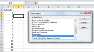
Figure 5. Screenshot of Sampling in Data Analysis menu, Microsoft Excel
Enter the cells with the numbers you wish to select from. In our example, column A has the numbers 1 through 26 representing each group in our class. I entered A:A as the Input Range.
Next, select “Random” and enter the number of samples. I want two.
Click OK and the output will be placed into cell B3 (my choice); I could have just as easily had Excel put the answer into a new worksheet.
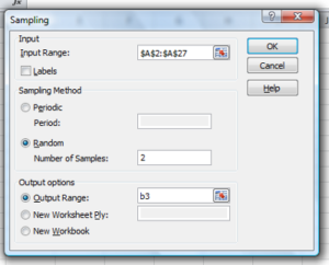
Figure 6. Screenshot of input required for Sampling in Data Analysis menu, Microsoft Excel
To sample with replacement from column A (with our 1 through 26), type in the formula B1
=INT(27*RAND())and the formula C1
=INDEX(A:A,RANK(B1,B:B))then drag the cell handles to fill in the columns (first column B, then column C).
That’ll do it for MS Excel or LibreOffice Calc.
Sampling with R (Rcmdr)
It’s much easier with much more control to get sampling in Rcmdr (R) than in Excel. Sampling in R is based on the function called sample() and sample.int(). I will present just the sample() command here.
sample(x, size, replace = FALSE, prob = NULL)Example
You want to sample ten integers between 1 and 10
sample(10)R output
sample(10)
[1]  5  1 10  8  7  3  4  9  2  6
You have a list of subjects, A1 through A10
subjects = c("A1","A2","A3","A4","A5","A6","A7","A8","A9","A10")
sample(subjects, 3, replace = FALSE, prob = NULL)
R output
sample(subjects, 3, replace = FALSE, prob = NULL)
[1] "A5" "A2" "A9"
Could use this to arrange random order for ten subjects
sample(subjects, 10, replace = FALSE, prob = NULL)
[1] "A9" "A3" "A8" "A2" "A1" "A4" "A10" "A7" "A5" "A6"
Try with replacement; To sample with replacement, type in TRUE after replace in the sample() function. The R output follows
sample(x, 10, replace = TRUE, prob = NULL)
[1]  5  5  3  5  3  7  3  5 10  6
R’s randomness is based on pseudonumbers and is, therefore, not truly random (actually, this is true of just about all computer-based algorithms unless they are based on some chaotic process). We can use this pseudo part to our advantage: if we want to reproduce our “random” process, we can seed the random number algorithm to a value (eg, 100), with the command in the Script Window
set.seed(100)For 10 random integers (eg, observations), type in the Script window
sample(10)R returns the following in the Output Window
sample(10)
[1] 4 5 7 3 10 9 2 1 6 8
Sampling was done without replacement. Here’s another selection round,
First without setting a seed value
sample(10)
[1] 10 4 7 3 8 1 2 9 6 5
Try again to see if get the same 10
sample(10)
[1]  1  4  8  2  9  6  5 10  3  7
Now to demonstrate how setting the seed allows you to draw repeated samples that are the same.
Note 3: If I need to precede the sample command with a set.seed() call, then sampling is repeatable.
set.seed(100)
sample(10)
[1] 4 3 5 1 9 6 10 2 8 7
and try again
set.seed(100)
sample(10)
[1] 4 3 5 1 9 6 10 2 8 7
Additional R packages that help with sampling schemes include: sampling() and spatialsample, which is part of the BiodiversityR package, which is available as a plugin for R Commander.
Quiz Chapter 5.6
Sampling from populations
Questions
- For our two descriptions of experiments in section 6.1 (the sample of patients; the sample of frogs), which sampling technique was used?
- What purpose is served by
set.seed()in a sampling trial? - Consider our question, Does taking a multivitamin daily improve health? Imagine you have a grant willing to support a long-term prospective study to follow up to one thousand people for ten years. List at least three concerns with proposed solutions about how sampling of subjects for the study.
- Imagine you wish to conduct a detailed survey to learn about student preferences. Your survey will include many questions, so you decide to ask just ten students. Student population is 70% female, 30% male.
- Assuming you select at random (simple random sampling), what is the chance that no male students will be included in your survey?
- You are able to increase the number of surveys to 20, 30, 40, or 50. What is the chance that no male students will be included in your survey for each of these increased sample numbers?
- What can you conclude about the effects of increasing survey sample size on representativeness of students for the survey?
- Discuss how you could apply a stratified sampling scheme to this survey and whether or not this approach improves representativeness.
- Why are random numbers generated by a computer called pseudo random numbers?
Chapter 5 contents
5.5 – Importance of randomization in experimental design
Introduction
If the goal of the research is to make general, evidenced-based statements about causes of disease or other conditions of concern to the researcher, then how the subjects are selected for study directly impacts our ability to make generalizable conclusions. The most important concept to learn about inference in statistical science is that your sample of subjects upon which all measurements and treatments are conducted, ideally should be a random selection of individuals from a well-defined reference population.
The primary benefit of random sampling is that it strengthens our confidence in the links between cause and effect. Often after an intervention trial is complete, differences among the treatment groups will be observed. Groups of subjects who participated in sixteen weeks of “vigorous” aerobic exercise training show reduced systolic blood pressure compared to those subjects who engaged in light exercise for the same period of time (Cox et al 1996). But how do we know that exercise training caused the difference in blood pressure between the two treatment groups? Couldn’t the differences be explained by chance differences in the subjects? Age, body mass index (BMI), overall health, family history, etc?
How can we account for these additional differences among the subjects? If you are thinking like an experimental biologist, then the word “control” is likely coming to the foreground. Why not design a study in which all 60 subjects are the same age, the same BMI, the same general health, the same family … history…? Hmm. That does not work. Even if you decide to control age, BMI, and general health categories, you can imagine the increased effort and cost to the project in trying to recruit subjects based on such narrow criteria. So, control per se is not the general answer.
If done properly, random sampling makes these alternative explanations less likely. Random sampling implies that other factors that may causally contribute to differences in the measured outcome, but themselves are not measured or included as a focus of the research study, should be the same, on average, among our different treatment groups. The practical benefits of proper random sampling is that recruiting subjects gets easier — fewer subjects will be needed because you are not trying to control dozens of factors that may (or may not!) contribute to differences in your outcome variable. The downside to random sampling is that the variability of the outcomes within your treatment groups will tends to increase. As we will see when we get to statistical inference, large variability within groups will make it less likely that any statistical difference between the treatment groups will be observed.
Demonstrate the benefits of random sampling as a method to control for extraneous factors.
The study reported by Cox et al included 60 obese men between the ages of 20 and 50. A reasonable experimental design decision would suggest that the 60 subjects be split into the two treatment groups such that both groups had 30 subjects for a balanced design. Subjects who met all of the research criteria and who had signed the informed consent agreement are to be placed into the treatment groups and there are many ways that group assignment could be accomplished. One possibility, the researchers could assign the first 30 people that came into the lab to the Vigorous exercise group and the remaining 30 then would be assigned to the Light exercise group. Intuitively I think we would all agree that this is a suspect way to design an experiment, but more importantly, why shouldn’t you use this convenient method?
Just for argument’s sake, imagine that their subjects came in one at a time, and, coincidentally, they did so by age. The first person was age 21, the second was 22, and so on up to the 30th person who was 50. Then, the next group came in, again, coincidentally in order of ascending age. If you calculate the simple average age for each group you will find that they are identical (35.5 years). On the surface, this looks like we have controlled for age: both treatment groups have subjects that are the same age. A second option is to sort the subjects into the two treatment groups so that a 21 year old is in Group A, and the other 21 year old is in Group B, and so on. Again, the average age of Group A subjects and of Group B subjects would be the same and therefore controlled with respect to any covariation between age and change in blood pressure. However, there are other variables that may covary with blood pressure, and by controlling one, we would need to control the others. Randomization provides a better way.
I will demonstrate how randomization tends to distribute the values in such a way that the groups will not differ appreciably for the nuisance variables like age and BMI differences and, by extension, any other covariable. The R work is attached following the Reading list. The take-home message: After randomly selecting subjects for assignment to the treatment groups, the apparent differences between Group A and Group B for both age and BMI are substantially diminished. No attempt to match by age and by BMI is necessary. The numbers are shown in the table and then in two graphics (Fig 1, Fig 2) derived from the table.
Table 1. Mean age and BMI for subjects in two treatment groups A and B where subjects were assigned randomly or by convenience to treatment groups.
| Group | Random assignment of subjects to treatment groups | Convenience assignment of subjects to treatment groups |
|---|---|---|
| A | 35.2 | 28 |
| B | 35.8 | 43 |
| A | 32.49 | 28.99 |
| B | 32.87 | 37.37 |
Just for emphasis, the means from Table 1 are presented in the next two figures (Fig 1 and Fig 2).
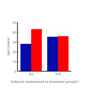
Figure 1. Age of subjects by groups (A = blue, B = red) with and without randomized assignment of subjects to treatment groups.
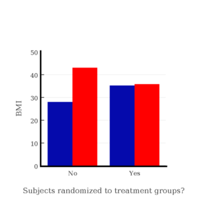
Figure 2. BMI of subjects by groups (A = blue, B = red) with and without randomized assignment of subjects to treatment groups.
Note that the apparent difference between A and B for BMI disappear once proper randomization of subjects was accomplished. In conclusion, a random sample is an approach to experimental design that helps to reduce the influence other factors may have on the outcome variable (eg, change in blood pressure after 16 weeks of exercise). In principle, randomization should protect a project because, on average, these influences will be represented randomly for the two groups of individuals. This reasoning extends to unmeasured and unknown causal factors as well.
This discussion was illustrated by random assignment of subjects to treatment groups. The same logic applies to how to select subjects from a population. If the sampling is large enough, then a random sample of subjects will tend to be representative of the variability of the outcome variable for the population and representative also of the additional and unmeasured cofactors that may contribute to the variability of the outcome variable.
What about observational studies? How does randomization work?
However, if you do cannot obtain a random sample, then conclusions reached may be sample-specific, biased. …perhaps the group of individuals that likes to exercise on treadmills just happens to have a higher cardiac output because they are larger than the individuals that like to exercise on bicycles. This nonrandom sample, an example of confounding where an extraneous or nuisance variable, body size, is associated with both the independent variable (exercise preference) and the dependent variable (cardiac output), will bias your results and can lead to incorrect interpretation of results.
Alternatively, perhaps a researcher elects to study the cardiac output of treadmill users versus bicycle users. The researcher sets up their testing station inside a gym’s powerlifting zone, where the largest individuals in the gym hang out. Inevitably because of this choice, the researcher over recruits larger individuals into the treadmill group, leading to a falsely elevated average cardiac output for treadmill users. This is an example of ascertainment bias — the sample is not representative of all treadmill users at the gym.
Random sampling is CRUCIAL in epidemiology, opinion survey work, most aspects of health, drug studies, medical work with human subjects. It’s difficult and very costly to do… so most surveys you hear about, especially polls reported from Internet sites, are NOT conducted using random sampling (included in the catch-all term “probability sampling“)!! As an aside, most opinion survey work involves complex sample designs involving some form of geographic clustering (eg, all phone numbers in a city, random sample among neighborhoods).
Random sampling is the ideal if generalizations are to be made about data, but strictly random sampling is not appropriate for all kinds of studies. Consider the question of whether or not EMF exposure is a risk factor for developing cancer (Pool 1990). These kinds of studies are observational: at least in principle, we wouldn’t expect that housing and therefore exposure to EMF is manipulated (cf. discussion Walker 2009). Thus, epidemiologists will look for patterns: if EMF exposure is linked to cancer, then more cases of cancer should occur near EMF sources compared to areas distant from EMF sources. Thus, the hypothesis is that an association between EMF exposure and cancer occurs non-randomly, whereas cancers occurring in people not exposed to EMF are random. Unfortunately, clusters can occur even if the process that generates the data is random.
Compare Graph A and Graph B (Fig 3). One of the graphs resulted from a random process and the other was generated by a non-random process. Note that the claim can be rephrased about the probability that each grid has a point, eg, it’s like Heads/Tails of 16 tosses of a coin. We can see clusters of points in Graph B; Graph A lacks obvious clusters of points — there is a point in each of the 16 cells of the grid. Although both patterns could be random, the correct answer in this case is Graph B.
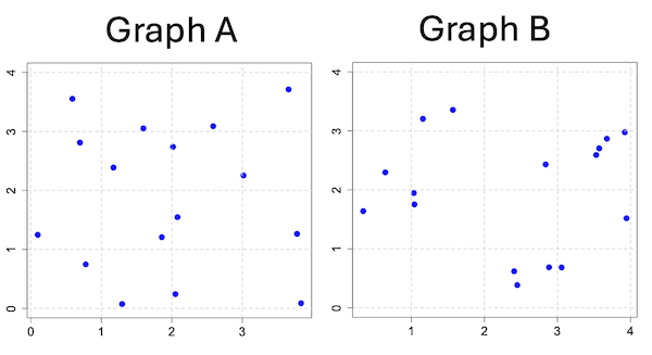
Figure 3. An example of clustering resulting from a random sampling process (Graph B). In contrast, Graph A was generated so that a point was located within each grid.
Hard to tell — and truth be told, random process could generate either one. To convince you, Figure 4 reveals the grouping that was done for Group A, in contrast with Group B which was drawn with the truly random process.
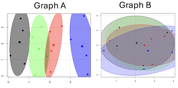
Figure 4. Same graphs as Figure 3, but with ellipses around the grouped data (hard to tell, but the centroids are the larger points).
Implications for sampling
The graphic below shows the transmission grid in the continental United States (Fig 5). How would one design a random sampling scheme overlaid against the obviously heterogeneous distribution of the grid itself? If a random sample was drawn, chances are good that no population would be near a grid in many of the western states, but in contrast, the likelihood would increase in the eastern portion of the United States where the population and therefore transmission grid is more densely placed.

Figure 5. Map of electrical transmission grid for continental United States of America. Image source https://openinframap.org/#3/24.61/-101.16
For example, you want to test whether or not EMF affects human health, and your particular interest is in whether or not there exists a relationship between living close to high voltage towers or transfer stations and brain cancer. How does one design a study, keeping in mind the importance of randomization for our ability to generalize and assign causation? This is a part of epidemiology which strives to detect whether clusters of disease are related to some environmental source. It is an extremely difficult challenge. For the record, no clear link to EMF and cancer has been found, but reports do appear from time to time (eg, report on a cluster of breast cancer in men working in office adjacent to high EMF, Milham 2004).
Questions
1. Use the sample() with and without replacement on the object (see help with R below)
fruit <- c("apple", "banana", "grape", "kiwi", "pear", "pineapple", "tomato")a) set of 3
b) set of 4
2. Confirm the claim by calculating the probability of Graph A result vs Graph B result (see R script below).
Quiz Chapter 5.5
Importance of randomization in experimental design
R code!
Code you type is shown in red; responses or output from R are shown in blue. Recall that statements preceded by the hash # are comments and are not read by R (ie, no need for you to type them).
First, create some variables. Vectors aa and bb contain my two age sequences.
 aa = seq(21,50)
 bb = seq(21,50)
Second, append vector bb to the end of vector aa
 age = append(aa,bb)
 age           #submit the vector (variable) name to print the records for verification - looks good!
  [1] 21 22 23 24 25 26 27 28 29 30 31 32 33 34 35 36 37 38 39 40 41 42 43 44 45 46 47 48 49 50 21 22 23 24 25 26 27 28 29 30 31 32 33 34 35 36 37
 [48] 38 39 40 41 42 43 44 45 46 47 48 49 50
Third, get the average age for the first group (the aa sequence) and for the second group (the bb sequence). Lots of ways to do this, I made a two subsets from the combined age variable; could have just as easily taken the mean of aa and the mean of bb (same thing!).
 A = age[1:30]
 mean(A)
 [1] 35.5
 B = age[31:60]
 mean(B)
 [1] 35.5
Fourth, start building a data frame, then sort it by age. Will be adding additional variables to this data frame
 ex.random = data.frame(age)
 AO.all = sort(ex.random$age)
 AO.age           #submit the vector (variable) name to print the records for verification - looks good!
  [1] 21 21 22 22 23 23 24 24 25 25 26 26 27 27 28 28 29 29 30 30 31 31 32 32 33 33 34 34 35 35 36 36 37 37 38 38 39 39 40 40 41 41 42 42 43 43 44
 [48] 44 45 45 46 46 47 47 48 48 49 49 50 50
Fifth, divide the variable again into two subsets of 30 and get the averages
 AO = AO.age[1:30]
 AO
  [1] 21 21 22 22 23 23 24 24 25 25 26 26 27 27 28 28 29 29 30 30 31 31 32 32 33 33 34 34 35 35
 mean(AO)
 [1] 28
 BO = AO.age[31:60]
 BO
  [1] 36 36 37 37 38 38 39 39 40 40 41 41 42 42 43 43 44 44 45 45 46 46 47 47 48 48 49 49 50 50
 mean(BO)
 [1] 43
Sixth, create an index variable, random order without replacement
rand.index = sample(1:60,60,replace=F)Add the new variable to our existing data frame, then print it to check that all is well
 ex.random$rand = rand.index
 ex.random
    age rand
 1   21   43
 2   22   15
 3   23   17
 4   24   35
 5   25   19
 6   26   18
 7   27   22
 8   28   31
 9   29   12
 10  30   44
 11  31   24
 12  32    5
 13  33    2
 14  34   50
 15  35   23
 16  36   20
 17  37   41
 18  38   56
 19  39   36
 20  40    8
 21  41   45
 22  42   38
 23  43   42
 24  44   46
 25  45   16
 26  46   21
 27  47   28
 28  48   10
 29  49   32
 30  50   54
 31  21   57
 32  22   51
 33  23   27
 34  24   40
 35  25   14
 36  26   48
 37  27   26
 38  28   58
 39  29    9
 40  30   11
 41  31    4
 42  32   52
 43  33   37
 44  34   53
 45  35    6
 46  36   34
 47  37   39
 48  38    7
 49  39    1
 50  40   47
 51  41   33
 52  42   60
 53  43   49
 54  44   30
 55  45   29
 56  46   55
 57  47   13
 58  48    3
 59  49   25
 60  50   59
Seventh, select for our first treatment group the first 30 subjects from the randomized index. There are again other ways to do this, but sorting on the index variable means that the subject order will be change too.
AR.age = ex.random[order(ex.random$rand),] #created a new data frame to distinguish it from the presorted version "ex.random"Print the new data frame to confirm that the sorting worked. It did. we can see that the rows have been sorted by ascending order based on the index variable.
 AR.age
    age rand
 49  39    1
 13  33    2
 58  48    3
 41  31    4
 12  32    5
 45  35    6
 48  38    7
 20  40    8
 39  29    9
 28  48   10
 40  30   11
 9   29   12
 57  47   13
 35  25   14
 2   22   15
 25  45   16
 3   23   17
 6   26   18
 5   25   19
 16  36   20
 26  46   21
 7   27   22
 15  35   23
 11  31   24
 59  49   25
 37  27   26
 33  23   27
 27  47   28
 55  45   29
 54  44   30
 8   28   31
 29  49   32
 51  41   33
 46  36   34
 4   24   35
 19  39   36
 43  33   37
 22  42   38
 47  37   39
 34  24   40
 17  37   41
 23  43   42
 1   21   43
 10  30   44
 21  41   45
 24  44   46
 50  40   47
 36  26   48
 53  43   49
 14  34   50
 32  22   51
 42  32   52
 44  34   53
 30  50   54
 56  46   55
 18  38   56
 31  21   57
 38  28   58
 60  50   59
 52  42   60
Eighth, create our new treatment groups, again of n = 30 each, then get the means ages for each group.
 AR = AR.age$age[1:30]
 mean(AR)
 [1] 35.16667
 AR2 = AR.all$all[31:60]
 mean(AR2)
 [1] 35.83333
Get the minimum and maximum values for the groups
 min(AR)
 [1] 22
 min(AR2)
 [1] 21
 max(AR)
 [1] 49
 max(AR2)
 [1] 50
Ninth, create a BMI variable drawn from a normal distribution with coefficient of variation equal to 20%. The first group with we will call cc
cc = rnorm(n=30,m=27.5, sd=5.5) #mean was 27.5 for this group with standard deviation of 5.5The second group called dd
dd = rnorm(n=30,m=37.5, sd=7.5) #mean was 37.5 for this group with standard deviation of 7.5Create a new variable called BMI by joining cc and dd
 BMI=append(cc,dd)
 BMI            #print out BMI to confirm. Looks good!
  [1] 27.87528 27.83250 31.88703 34.99041 24.06751 23.50952 22.57779 31.48394 31.04321 25.60258 25.41081 22.34619 34.62213 36.41348 41.17740
 [16] 20.56529 27.25238 21.85205 32.11690 32.37168 23.11314 33.29110 34.99106 38.22016 18.72105 26.22030 25.13412 27.50475 34.79361 32.81267
 [31] 47.57872 27.58428 40.17211 38.22195 26.91893 37.02784 53.72671 34.94727 30.35245 38.32571 40.52111 36.15627 30.36592 36.20397 47.63142
 [46] 40.30846 36.47643 50.86804 43.63741 37.84994 42.82665 41.71008 28.44976 24.57906 42.37762 38.38512 35.22879 31.34063 34.02996 27.28038
Add the BMI variable to our data frame.
 ex.random$BMI = BMI
 ex.random              #Print out the revised data frame. Looks good. We now have three variables: age, the index "rand," and now BMI
    age rand      BMI
 1   21   43 27.87528
 2   22   15 27.83250
 3   23   17 31.88703
 4   24   35 34.99041
 5   25   19 24.06751
 6   26   18 23.50952
 7   27   22 22.57779
 8   28   31 31.48394
 9   29   12 31.04321
 10  30   44 25.60258
 11  31   24 25.41081
 12  32    5 22.34619
 13  33    2 34.62213
 14  34   50 36.41348
 15  35   23 41.17740
 16  36   20 20.56529
 17  37   41 27.25238
 18  38   56 21.85205
 19  39   36 32.11690
 20  40    8 32.37168
 21  41   45 23.11314
 22  42   38 33.29110
 23  43   42 34.99106
 24  44   46 38.22016
 25  45   16 18.72105
 26  46   21 26.22030
 27  47   28 25.13412
 28  48   10 27.50475
 29  49   32 34.79361
 30  50   54 32.81267
 31  21   57 47.57872
 32  22   51 27.58428
 33  23   27 40.17211
 34  24   40 38.22195
 35  25   14 26.91893
 36  26   48 37.02784
 37  27   26 53.72671
 38  28   58 34.94727
 39  29    9 30.35245
 40  30   11 38.32571
 41  31    4 40.52111
 42  32   52 36.15627
 43  33   37 30.36592
 44  34   53 36.20397
 45  35    6 47.63142
 46  36   34 40.30846
 47  37   39 36.47643
 48  38    7 50.86804
 49  39    1 43.63741
 50  40   47 37.84994
 51  41   33 42.82665
 52  42   60 41.71008
 53  43   49 28.44976
 54  44   30 24.57906
 55  45   29 42.37762
 56  46   55 38.38512
 57  47   13 35.22879
 58  48    3 31.34063
 59  49   25 34.02996
 60  50   59 27.28038
Tenth, repeat our protocol from before: Set up two groups each with 30 subjects, calculate the means for the variables and then sort by the random index and get the new group means.
 AO = ex.random$BMI[1:30]
 mean(AO)
 [1] 28.99333
 BO = ex.random$BMI[31:60]
 mean(BO)
 [1] 37.36943
All we did was confirm that the unsorted groups had mean BMI of around 27.5 and 37.5 respectively. Now, proceed to sort by the random index variable. Go ahead and create a new data frame
 AR.age = ex.random[order(ex.random$rand),]
 AR.age                 #Print out the new data frame to confirm. Looks good.
    age rand      BMI
 49  39    1 43.63741
 13  33    2 34.62213
 58  48    3 31.34063
 41  31    4 40.52111
 12  32    5 22.34619
 45  35    6 47.63142
 48  38    7 50.86804
 20  40    8 32.37168
 39  29    9 30.35245
 28  48   10 27.50475
 40  30   11 38.32571
 9   29   12 31.04321
 57  47   13 35.22879
 35  25   14 26.91893
 2   22   15 27.83250
 25  45   16 18.72105
 3   23   17 31.88703
 6   26   18 23.50952
 5   25   19 24.06751
 16  36   20 20.56529
 26  46   21 26.22030
 7   27   22 22.57779
 15  35   23 41.17740
 11  31   24 25.41081
 59  49   25 34.02996
 37  27   26 53.72671
 33  23   27 40.17211
 27  47   28 25.13412
 55  45   29 42.37762
 54  44   30 24.57906
 8   28   31 31.48394
 29  49   32 34.79361
 51  41   33 42.82665
 46  36   34 40.30846
 4   24   35 34.99041
 19  39   36 32.11690
 43  33   37 30.36592
 22  42   38 33.29110
 47  37   39 36.47643
 34  24   40 38.22195
 17  37   41 27.25238
 23  43   42 34.99106
 1   21   43 27.87528
 10  30   44 25.60258
 21  41   45 23.11314
 24  44   46 38.22016
 50  40   47 37.84994
 36  26   48 37.02784
 53  43   49 28.44976
 14  34   50 36.41348
 32  22   51 27.58428
 42  32   52 36.15627
 44  34   53 36.20397
 30  50   54 32.81267
 56  46   55 38.38512
 18  38   56 21.85205
 31  21   57 47.57872
 38  28   58 34.94727
 60  50   59 27.28038
 52  42   60 41.71008
Get the means of the new groups
 AR = AR.age$BMI[1:30]
 mean(AR)
 [1] 32.49004
 min(AR)
 [1] 18.72105
 max(AR)
 [1] 53.72671
 AR2 = AR.all$BMI[31:60]
 mean(AR2)
 [1] 33.87273
 min(AR2)
 [1] 21.85205
 max(AR2)
 [1] 47.57872
That’s all of the work!
Data set
nonrandom
| X | Y |
| 0.779 | 0.747 |
| 0.098 | 1.248 |
| 0.697 | 2.811 |
| 0.59 | 3.553 |
| 1.295 | 0.075 |
| 1.858 | 1.207 |
| 1.172 | 2.388 |
| 1.597 | 3.051 |
| 2.051 | 0.242 |
| 2.081 | 1.546 |
| 2.016 | 2.738 |
| 2.587 | 3.088 |
| 3.833 | 0.088 |
| 3.776 | 1.264 |
| 3.017 | 2.254 |
| 3.657 | 3.712 |
random
| X1 | Y1 |
| 1.157 | 3.203 |
| 2.407 | 0.62 |
| 1.033 | 1.946 |
| 3.676 | 2.866 |
| 3.57 | 2.703 |
| 3.056 | 0.685 |
| 1.568 | 3.355 |
| 1.041 | 1.753 |
| 0.643 | 2.295 |
| 2.884 | 0.687 |
| 3.53 | 2.591 |
| 2.838 | 2.431 |
| 3.945 | 1.518 |
| 0.34 | 1.64 |
| 2.45 | 0.386 |
| 3.921 | 2.976 |
Chapter 5 contents
- The basics explained
- Experiments
- Experimental and Sampling units
- Replication, Bias, and Nuisance Variables
- Clinical trials
- Importance of randomization in experimental design
- Sampling from Populations
- References and suggested readings
5.4 – Clinical trials
Introduction
Two areas of inquiry have contributed enormously to our understanding of experimental design: agriculture research (Verdooren 2020) and human subject clinical trials. This page outlines types of clinical trial designs and briefly introduces the subject of research ethics with human subject research (Huang and Hadian 2006). After completing this page, the reader will be able to identify key clinical trial types and recognize the fundamental ethical principles governing human subject research.
Although this page does not address the many concerns for ethical research in ecology and environmental studies, many parallels can be drawn (Crozier and Schulte-Hostedde 2014, Samuel and Richie 2022). To name just one example, both disciplines mandate a “do no harm,” principle. In clinical research this amounts to minimizing risks to human subjects; in environmental and ecology studies, acknowledging experimental studies through sampling or chemical releases can damage ecosystems (Resnik 2009).
An outline of clinical trials
Much has been written about biomedical research study design; a couple of accessible articles that can supplement the material presented here include Benson and Hart 2000, Concato et al 2000, Gabriella 2012. Even if you never work in clinical research, understanding how clinical trials are designed and under what circumstances limitations of particular designs arise is helpful to all of us who do experimental work. In Mike’s Workbook for Biostatistics we will present descriptions of research activities and step through situations where you will attempt to align the research by analogy to clinical trials. A second approach to learning about experimental design is to read about someone’s study, and reworking it in terms of a clinical trial design perspective. We will use a discussion of clinical trials, used in biomedical research to investigate effectiveness of treatments of disease, as our starting point for learning how statistics informs experimentation.
Types of clinical trials are distinguished by their design and include:
Case studies are a thorough analysis of an individual patient, or a few individuals (a group), focusing on symptoms, diagnostics, treatments and outcomes. Case studies can utilize quantitative or qualitative research methods. Case studies, of course, are not restricted to medical research. The main disadvantage of case studies is that by definition they are not generalizable to the population and, by their very nature, researcher subjectivity (choice of diagnostics, interpretations) and other kinds of bias may be challenging to control. A 2025 case study received considerable news coverage: a 60 year old man developed bromism — a toxic condition resulting from excessive exposure to bromides — consulting ChatGPT for health information (Eichenberger et al 2025).
Experimental studies are just that, research designs that apply techniques of experimental science — controls, randomization, attempts to account for sources of bias. They are intended to make direct comparisons among subjects assigned by the researcher to treatment groups. By definition experiments are longitudinal studies. Longitudinal studies are experimental or observational studies in which multiple observations are recorded for each individual and individuals are tracked over time. Many excellent resources about experimental design, beginning with R.A. Fisher’s 1935 book, The design of experiments, to Scheiner and Gurevitch (Editors) 2001, Design and Analysis of Ecological Experiments (2nd edition), to the many books on randomized control trials, eg, the 5th edition of Designing clinical research (2022), edited by Browner et al.
Observational (or epidemiological) studies — no direct intervention is administered and so observational studies tend to be retrospective; we identify individuals with and without the condition and attempt to identify associations between the condition and any number of potential causal factors.
Cross-sectional studies are examples of descriptive study designs. They take observations at one point in time on a variety of individuals. It can be used to associate factors with the condition in question, and can be used to estimate the prevalence of a condition in the population. Omair (2015) provides an accessible summary of case and cross-sectional study designs.
Cross-sectional studies are referred to as method = cross.sectional in the package epiR.
Cohort studies involve a group of subjects (eg, patients) who receive the same treatment at the same time. A cohort consists of subjects who are linked in some way. It could be a trivial link, like the cohorting done at university (all incoming Freshmen students who enroll for a class offered at 9:30AM), or it could be based on shared experience due to an exposure event (eg, all passengers on a jet traveling with an index case or “patient zero”).
- Prospective cohort studies enroll people as cohorts at the beginning of a study and follow them over time
- Retrospective cohort studies may utilize archived records.
Cohort and other variations of observational studies (eg, case control, test-negative design), can establish associations between risk factors and conditions or specific adverse events, but cannot by themselves establish cause and effect (Benson and Hartz 2000). A search of PUBMED for “cohort study” reports more than 3.2 million studies since 1914. A 2025 prospective cohort study with more than 1800 pregnant women found no change in risk of major birth defects after maternal mRNA COVID-19 vaccination in the first trimester of pregnancy (Kayser et al 2025).
Cohort studies are referred to as method = cohort.count in the package epiR.
Case control studies are similar to cohort studies, except they are retrospective. Case refers to subjects with one or more characteristics of interest. Used to infer the exposure risk factor by evaluating historical records. Omair (2016) provides an accessible summary of cohort and case control study designs. Designed to identify associations between exposure and particular outcomes, case control studies are retrospective and observational studies: Retrospective because the outcomes are already known, and observational because the event was caused by nature, not experiment. In principle, researchers identify a number of cases with a particular outcome (eg, lung cancer), then attempt to match cases to individuals who do not have the outcome (controls). Work is done to look back to see if the exposure (eg, smoking) is more frequent in the case group than the control group.
Case control studies have several advantageous compared to other approaches: rapid to conduct compared to longitudinal studies (the even has already happened), and efficient because small sample sizes may be enough to reach conclusions. Among their limitations, however, is the problem of how to match cases with controls. Obvious matching accomplished by grouping by age categories, body mass index, gender, socio-economic status, and so on. Three papers authored by Wacholder published in American Journal of Epidemiology 1992 describe in detail, from theory to practice, case control selection (Wacholder 1992abc). A search of PUBMED for “case control” reports more than 400 thousand studies since 1950. A 2025 case control study with more than one million records found no effect of aluminum adjuvant in childhood vaccines on chronic autoimmunity, atopy or allergy, and neurodevelopmental disorders (Andersson et al 2025).
Case control studies are referred to as method = case.control in the package epiR.
Test-negative designs are a kind of case control studies where the cases are those testing positive for the specific agent and controls are those who test negative for the agent, but importantly, both groups are individuals seeking care for symptoms characteristic of exposure to the agent (Kissling et al 2009, Fukushima and Hirota 2017). This design is intended to reduce the effects of health-care seeking behavior, therefore minimizing possible selection bias, and, therefore false associations between exposure and disease. Note however, that test-negative studies rely on test accuracy (discussed in Chapter 7.3 – Conditional Probability and Evidence Based Medicine); false negatives, where a person has the disease but test results return negative, incorrectly assigns the individual to the control group. This leads to underestimation of true effect of the intervention, eg, vaccination Fukushima and Hirota 2017).
Randomized Control (interventional or experimental) Trials (RCT): compares an experimental treatment group with a control) placebo group. The groups are assigned to groups randomly. Another variant of a RCT is a randomized clinical trial, with the only difference that the clinical trial compares different treatments and may not include a control group.
Double-blind: The “gold standard” RCT. Both the patient and those interacting with the patient do not know what treatment the patient has received.
Placebo: a treatment in name only. The placebo is a designed but medically ineffective agent given to a study subject. There is considerable debate about what a placebo should contain and as to the ethics and general merits of its use in clinical trials (Temple and Ellenberg 2000).
- active control or comparator studies are now common in place of placebo studies where treatment is clearly better than not giving the subject something of benefit (i.e., the placebo which is designed to not benefit the subject). Active control is not automatically a better choice than placebo control because they may be less effective in evaluating cause and effect (Temple and Ellenberg 2000).
The controlled clinical trial has a long history: Daniel’s vegetarian diet (Daniel’s training in Babylon, Book of Daniel, Old Testament, discussed in Bhatt 2010, h/t Treece 1990) — after ten days those on Daniel’s diet looked healthier than the others who ate the King’s prescribed meal of meat and wine; James Lind’s scurvy trials on board HMS Salisbury British ship in 1747 (references in Bhatt 2010). Randomized control trials (RCT) were introduced by Hill and others in 1946 study of streptomycin efficacy against tuberculosis. The effectiveness of RCT are now established and integral to regulation of drug development.
Use of clinical trials unfortunately has a longer history than recognition of human rights (Rice 2008). World War II Nazi medical research atrocities are well known (Berger 1990), so too the longitudinal study of Tuskegee syphilis study on African-Americans (Brandt 1978). But there are too many other examples: 1884 Hawaii, inoculation of Keanu by Dr. Arning with leprosy in exchange for commuting Keanu’s death sentence to life imprisonment (Keanu developed leprosy and died in 1890, Binford 1936); many studies of American Indians/Alaskan natives (Hodge 2012). Concerns about ethical treatment of participants in studies remains a challenge; see controversy over prospective randomized control trial (NCT00078182) of safety and efficacy of an HIV prophylactic tenofovir treatment in Cambodia (Singh and Mills 2005, Mills et al 2005).
Rules of conduct were established at Nuremberg, and subsequently extended and codified by Belmont Accords: core principles of respect for persons, beneficence, and justice. Ethical standards of who participates are institutionalized by IRB boards. True informed consent remains challenging (Rothwell et al 2021 and references therein).
Figure 1 shows how common in PUBMED randomized control trials and references to use of double blind design in research (Fig 1).
Figure 1. Search of PUBMED for “RCT” and “double blind” studies from 1950 to 2024.
Ethics of clinical and experimental research
Informed consent of subjects before proceeding in a clinical trial is a required, essential component of the design of a clinical trial. Guidelines for research conducted on human subjects originated from The Nuremberg Code (Shuster 1997). The Code was formulated 67 years ago, in August 1947, in Nuremberg, Germany, by American judges sitting in judgment of Nazi doctors accused of conducting torturous experiments on humans in the concentration camps (Shuster 1997). It served as a blueprint for today’s principles that ensure the rights of subjects in medical research. Achieving informed consent is not always straightforward (Nijhawan et al 2013), and we continue to see research that challenges ethical standards (eg, discussion in Suba 2014). Additionally, and perhaps less appreciated, the Nuremberg Code is justification for invasive animal research: animal research must precede human subject testing (Shuster 1997).
While informed consent is required, clearly, it is not enough. Emmanuel et al (2000) provide a framework for evaluating the ethics of a research program involving human subjects:
- Value
- Scientific validity
- Fair subject selection
- Favorable risk-benefit ratio
- Independent review
- Informed consent
- Respect for enrolled subjects
An additional concept, clinical equipoise (Freedman 1987) is relevant. Freedman noted that the researcher must have “genuine uncertainty” with respect to the merits of each treatment, or an “honest null hypothesis.” If a consensus exists that one treatment is better than another, including placebo, then there is no null hypothesis and the research would be invalid (Emmanuel et al 2000). Take, for example, the suggestion that clinicians should withhold angiotensin converting inhibitors (ACE2) from their hypertensive Covid-19 patients (Fang et al 2020; discussed in Tignaneli et al 2020). The hypothesis comes from the observation that SARS-COV2, like SARS-Cov, binds with ACE2 receptor in order to invade the cell. Blocking ACE2 inhibitors then would reduce activation of pulmonary renin angiotensin system and subsequent lung injury. Tignaneli et al (2020) called this a case of clinical equipoise — they argued no evidence supports “routine discontinuation” of ACE inhibitors.
Returning to the framework, Emmanuel et al left the equipoise consideration off their list for a number of reasons — for example, clinical equipoise can lead researchers to view pursuit of research has the same weight as therapy. Importantly, the proposed framework shifts the focus from the researcher views to a structured process of oversight that may minimize exploitation. It emphasizes factors like independent review and informed consent as more reliable ethical safeguards.
Moreover, the Nuremberg Code is foundational but not the current, nor the sole guidance for research conducted on human subjects; modern biomedical research is guided by more comprehensive documents like the Declaration of Helsinki and the Belmont Report, in addition to federal regulations and Institutional Review Boards or IRB.
Guidelines mandate detail about experimental design.
Professional journals expect authors to provide detailed descriptions of all methodology, including aspects of experimental design. Fundamental to the aim of science, to increase our knowledge An essential component of science To improve this kind of communication many journals and professional societies have promoted standards about what must be included in these descriptions. For example, efforts of the CONSORT, which stands for CONsolidated Standards Of Reporting Trials, at www.consort-statement.org, to improve the reporting of clinical trials by authors and provide guidelines for reviewers and editors is endorsed by more than 400 journals. The CONSORT checklist address
- Trial design
- Participants
- Interventions
- Outcomes
- Sample size
- Randomization
- Implementation
- Blinding
- Statistical methods
These nine elements were judged essential for authors to report how their study implemented or did not implement. The purpose of these items is to in order to improve reproducibility of published research. For animal research a similar list is available from ARRIVE (Kilkenny et al 2010). ARRIVE also addresses additional criteria and directs how these should be reported throughout the paper, not just in the methods section. Like CONSORT, hundred of journals have endorsed the ARRIVE 20-item checklist.
Clinical researchers must implement protocols to insure data management guidelines are followed. Clinical data management is a large topic in and of itself, so we won’t discuss this area further. However, good data management practice across disciplines share a number of features. For example, all data records should include metadata, where metadata refers to “information about data,” and would include enough information about the experiment, including
- dates and times of observations
- personnel
- facilities
- protocols used
- number of subjects
- list of variables with definitions
- full name of variable plus any acronym
- measurement units
- instrumentation
- notes about data quality
- conditions
and more (this is hardly an exhaustive list). Metadata therefore explains how data were obtained. Lists of variables are also called data dictionaries. If data are stored in spreadsheets, for example, then good practice includes including a worksheet with the metadata for the data set.
Note 1: We introduced metadata and data dictionaries with our discussion about data types in Chapter 3.1.
Questions
- Be able to define the following terms
- case control
- case study
- cohort study
- cross sectional study
- observational study
- experimental study
- single arm trial
- single blind vs double-blinding in research design
- Early in the Covid-19 pandemic, hydroxycholoquine was suggested for treating Covid-19 patients, and some called for prophylactic use of the malarial drug. Discuss the treatment hypothesis in the context of clinical equipoise.
- Distinguish between case control prospective and case control retrospective studies and the kinds of inferences that can be made.
Quiz Chapter 5.4
Clinical trials
Chapter 5 contents
5.3 – Replication, Bias, and Nuisance Variables
Introduction
This page describes additional elements of experimental design, replication and bias, which can impact the validity of a study.
Replication in science refers to repeating an experiment under identical conditions multiple times. To the extent the same conclusions are achieved, we can say the outcome is reproducible (Simmons 2014) and, therefore, likely to be objectively true (Earp 2011). Replication of experimental and sampling units is an essential component of good experimental design. Confusing technical replicates for biological replicates is called pseudoreplication.
Bias refers to any of a number of sociological and cognitive errors which may influence conclusions in science (Ionnidis 2005). In a meta-analysis, Fanelli et al (2017) reported that while the size of effect from identifiable biases were small, some disciplines were more prone to these sources of error. That researchers testing similar hypotheses reach different conclusions may result from bias. One such bias is positive outcome bias, where reports of null hypotheses are more often rejected than they should be based on sample size and other concerns of statistical power (see Chapter 11 – Power analysis).
The page concludes with a discussion of nuisance variables, variables that may be causally associated with the outcome of interest, but themselves are either of no interest in the study, or may not be known in advance (Meehl 1970; see also discussion of spurious correlations in Chapter 16.3 – Data aggregation and correlation).
Technical vs. biological replicates.
A laboratory technician retrieves a vial of an immortalized cell line from cryostorage and initiate propagation of the cells for the week’s work. After a couple of days of subculturing, the technician has grown millions of cells and is ready to set up an assay. After washing the cells in PBS (phosphate buffered saline), the technician adjusts the concentration of cells to 10,000 per mL media, places the tube on ice, and proceeds to set up a 48 well microplate. To each well, the technician adds media, one or more agents (Table 1), plus cells, total volume each well at one mL, three replicates per treatment.
Table 1. In our example there were four treatments plus a control (media only)
- DMSO only (D)
- DMSO + Cytokine (DC)
- DMSO + Small molecule Inhibitor (DS)
- DMSO + Cytokine + Small molecule Inhibitor (DCS)
- Media only (M)
The plate table might look something like Figure 1.

Figure 1. Schematics of a set up for a hypothetical 48 well microplate (plate_plot() from ggplate package).
The technician has done a lot of work; but, from a statistician’s point of view, effectively the technician has but one sampling unit to show for his efforts; one biological sampling unit because as far as we can tell, the cells were all related. Biological replication refers to repeat measures (eg, same conditions) on biologically distinct entities (Blainey et al 2014). Technical replication, in contrast, refers to repeat measures on the same entity, eg, the same individual (Blainey et al 2014).
However, there were more than one technical samples in the experimental design, twelve in all because there were twelve wells. Many of you will recognize this as the distinction between technical and biological replicates. In thinking about experimental design replicates pertain to the number of sampling units that are treated the same way. In our example cells may be “treated the same way” in at least two distinct ways. Biologically, the cells may be the same: derived from the same clonal cell, all at the same passage (generation) number, each cell genetically, morphologically, physiologically (etc.,) identical to the next cell. Technical replication on the other hand pertains to the levels of the treatments.
Within each of these treatments we had three wells, and that’s at the level of the technical replication.
A final note on this experiment. We as molecular biologists call each of these treatment groups, but statisticians thinking of this design would recognize only one treatment (called in statistics a factor), with four levels of the treatment. We will discuss this beginning in chapter 12 when we introduce analysis of variance.
Types of bias.
When we make decisions, we like to think we are rational; that we make decisions based on an evaluation of evidence. And yet, an increasing body of literature suggests that our decisions often made in a manner that falls short of rational processing. We outlined some sources of bias in Chapter 2.6. Deviance from rational decision making is due to any number of cognitive biases we may have. Researchers and medical doctors make many decisions and, unfortunately, are just as susceptible to cognitive biases as the rest of us. One kind of bias that is bedeviling to research is confirmatory bias. Confirmatory bias refers to a researcher in effect seeking evidence in a way that confirms a prior conclusion (Kaptchuck 2003). Confirmatory bias would be exhibited if we report positive effects of aspirin to relieve migraines in subjects, but exclude cases where the subjects report no improvement. Medical doctors may be risk averse and therefore tend to over-prescribe, or they may be risk-takers (eg, rise and fall of high-dose chemotherapy, cf, discussion in Howard et al. 2011).
The concept of bias was first introduced in Chapter 3 and will be returned to in subsequent chapters. In general, bias refers to the objectivity of measurement and inferences about such measurements. Bias implies that a series of measurements consistently fail to return the true value of the variable. Bias is systematic error and may be associated with a poorly calibrated instrument or even the use of improper sets of rules for measurement given the nature of the characteristic. Bias can be captured by the concept of accuracy.
Bias is challenging to eliminate; the best way is to design the experiment so that the observer, the researcher, is unaware of the specific questions to be tested. The research is conducted “blind.” Clinical research provides the easiest examples. A trial can be blind in a couple of ways:
- The subjects do not know which treatment they receive, but the researcher does know
- The researcher does not know which treatment subjects receive, but the subjects know
- Neither the researcher nor the subjects know which treatment they receive.
- The other possibility is that both the researcher and the subjects know treatments received — this would be a poor design.
Bias can enter a research project at multiple levels. A partial list of sources of bias in research includes (modified after Pannucci and Wikins 2010):
Bias that occurs before the experiment
- Inadequate planning of the experiment, flawed design
- Bias in selection of subjects from the reference population
- Surveillance bias, where one group is studied more closely than another group.
Surveillance bias, also called detection bias or ascertainment bias, a type of information bias. Characterized as “the more you look, the more you find (Sackett 1979),” differences in outcome counts varies with differences in effort to detect. Recently, cases of myocarditis in young people were reported following Covid-19 mRNA vaccination (eg, Bozkurt et al 2021. Marshall et al 2021). However, myocarditis reports following vaccination occur at the rates expected in the population, and the reports lack important context (eg, other respiratory viruses known to cause myocarditis not ruled out), suggesting the putative link between Covid-19 vaccines and this heart condition may be result of us looking hard for signs of adverse effects of the vaccine (cf, discussion in O’Leary and Maldonado 2021).
Bias during the experiment
- Interviewer bias
- Chronology bias
- Recall bias
- Transfer bias
- Misclassification of exposure or outcome
- Performance bias
Performance bias refers to conditions of an experiment that introduce unintended differences between groups. For example, subjects enrolled in a weight-loss study randomly assigned to the control group may react poorly when they realize they are not receiving the experimental intervention. This leads to potential for a systematic bias — participants in the control group may behave differently, counteracting the point of randomization (McCambridge et al 2014).
Another well-known performance bias is associated with eliciting maximal performance from animals, such as running stamina or maximum sprint running speed (Losos et al 2002). For example, spring running speed of lizards may be measured by placing lizards onto a high-speed treadmill, then increasing belt speed to match the individual’s burst performance (eg, Dohm et al 1998). Clearly, not all individuals will perform to maximum physiological capabilities under these conditions.
Bias after the experiment
- Citation bias
- Confounding
Another way to view sources of bias is that, at least from the perspective of the researcher, the bias is likely to be unconscious bias. After all, if we knew about the sources of bias we would work our experiments in such a way to minimize known error producing sources (Holman et al 2015). Selecting subjects at random and keeping record keeping blind with respect to treatments are among the best tools we have to avoid this kind of bias.
Nuisance variables
A key quality of experimental design is the opportunity afforded the researcher to apply control. In a classic view of the experiment, one allows only one aspect to vary, the treatment applied, all else is controlled. Thus, any difference in outcome may be attributed to the treatment. However, it is likely impossible to control for all possible variables that may affect our outcome; confounding clear interpretation of results (see Chapter 16.2 and 16.3). Consider, for example, the effects of age on running performance (Fig. 2).
Figure 2. Mean 5K running times (minutes) by age and gender (2006 – 2016, Jamba Juice Banana 5K race, Honolulu, HI).
If we are interested in gender differences, we must also deal with the change in performance with age: older runners regardless of gender tend to run slower than younger runners. Thus, in the comparison of genders, age is a nuisance variable. In the literature, you may see “lurking variable,” or other such names. The concept is that these variables may be causal, but are either of no interest in the study, or may not be known in advance. Therefore, age must be accounted for before we can address gender differences, if any. Age, in this case, is considered a nuisance variable because we are not primarily interested in age effects, but age clearly covaries (is associated) with running performance. How best to handle nuisance variables? One approach is to match by age (blocking effect, see Chapter 14.4); another approach would be to randomly select with respect to age when compiling female and male times.
Another example of confounding. Results from ecological experiments intended to test for presence of competition for resources by plant species by removing plants may alter herbivory levels; thus, survivorship not the result of reduced plant-plant competition but because of changes in herbivore behavior (Reader 1992).
Questions
- I cite a number of articles in Mike’s Biostatistics Book. If you’re paying attention, you’ll have noticed that all of my citations, at least for articles, link to a source that you can either download or read online. What kind of error am I committing by following this approach?
- In large part because of the tendency for overuse of antibiotics, doctors are less likely today to prescribe antibiotics for patients with upper respiratory tract infections than in the past (Zoorob et al 2012). URTI are mostly caused by rhinovirus infections (Calderaro et al 2022) and, therefore, the course of infection in a patient should be unaffected by addition of antibiotic. However, although rare compared to URTI, life-threatening illness like acute epiglottitis caused by bacteria infection can sometimes develop or accompany URTI. Thus, not prescribing antibiotics at a diagnosis of URTI may risk a worsening condition for the patients. This sets the doctor up for a potential cognitive bias – to prescribe or not to prescribe antibiotics prophylactically? Discuss this decision in the context of potential sources of cognitive biases and possible outcomes of the decision.
Quiz Chapter 5.3
Replication, bias, and nuisance variables
Chapter 5 contents
- The basics explained
- Experiments
- Experimental and Sampling units
- Replication, Bias, and Nuisance Variables
- Clinical trials
- Importance of randomization in experimental design
- Sampling from Populations
- References and suggested readings
5.2 – Experimental units, Sampling units
Introduction.
Sampling units refer to the measured items, the focus of data collection; samples are selected from populations. Often, sampling units are the same thing as individuals. For example, if we are interested in the knowing whether men are more obese than women in Hawai’i, we would select individuals from the population; we would measure individuals. Thus, the sampling unit would be individuals, and the measurement unit would be percent body fat recorded for each individual. The data set would be the collection of all body fat measures for all individuals in the study, and we would then make inferences (draw conclusions) about the differences, if any, between adult males and females for body fat.
But sampling units can also refer to something more restrictive than the individual. For example, we may be interested in how stable, or consistent, is a person’s body fat over time. If we take a body fat measure once per year over a decade on the same group of adults, then the sampling unit refers to each observation of body fat recorded (once per year, ten times for an individual), and the population we are most likely to be referring to is the collection of all such readings (ten is arbitrary — we could have potentially measured the same individual thousands of times).
In some cases the researcher may wish to compare groups of individuals and not the individuals themselves. For example, a 2001 study sought to see if family structure influenced the metabolic (glycemic) control of children with diabetes (Thompson et al 2001). The researchers compared how well metabolic control was achieved in children of single parents and two-parent families. Thus, the sampling units would be families and not the individual children.
Experimental units.
Experimental units refers to the level at which treatments are independently applied in a study. Often, but not always, treatments are applied directly to individuals and therefore the sampling units and experimental units in these cases would be the same.
Question 1: What is the sampling unit in the following cell experiment?
A technician thaws a cryo tube containing about ½ million A549 cells (Foster et al 1998) and grows the cells in a T-75 culture flask (the 75 corresponds to 75 cm2 growing area) in a CO2 incubator at 37 °C. After the cells reach about 70% confluency, which may represent hundreds of thousands of cells, the technician aliquots 1000 cells into twelve wells of a plate for a total of 12000 cells. To three wells the technician adds a cytokine, to another three wells he adds a cytokine inhibitor, and to another three wells he adds both the cytokine and it’s inhibitor, and to the last three wells he adds DMSO, which was the solvent for both the cytokine and the inhibitor. He then returns the plate to the incubator and 24 hours later extracts all of the cells and performs a multiplex quantitative PCR to determine gene expression of several target genes known to be relevant to cell proliferation.
The described experiment would be an example of a routine, but not trivial procedure the technician would do in the course of working on the project in a molecular biology laboratory.
The choices for numbers provided in the description we may consider for the number of sampling units are:
- 1000 cells
- 12,000 cells
- ½ million cells
- 3 wells
- 12 wells
- The target genes
- None of the above
The correct answer is G, None of the above.
“None of the above” because the correct answer is … there was just one sampling unit! All cells trace back to that single cryo tube.
To answer the question, start from the end and work your way back. What we are looking for is independence of samples and at what level in the experiment we find independence. Our basic choice is between numbers of cells and numbers of wells. Clearly, cells are contained in the wells, so all of the cells in one well share the same medium, being treated the same way, including all the way back to the cryo tube — all of the cells came from that one tube so this lack of independence traces all the way back to the source of the cells. Thus, the answer can’t be related to cell number. How many wells did the technician set up? Twelve total. So, the maximum number of sampling units would be twelve, unless the samples are not independent. And clearly the wells (samples) are not independent because, again, all cells in the twelve wells trace back to a single cryo tube. Thus, from both perspectives, wells and cells, the answer is actually just one sampling unit! (Cumming et al 2007; Lazic 2010). Finally, the genes themselves are the targets of our study — they are the variables, not the samples. Moreover, the same logic applies — all copies of the genes are in effect descended from the few cells used to start the population.
Experimental and sampling units often, but not always the same.
Question 2: What is the experimental unit in the described cell experiment?
- 1000 cells
- 12,000 cells
- ½ million cells
- 3 wells
- 12 wells
- The target genes
- None of the above
The correct answer is E, 12 wells. Noted above, the technician applied treatments to 12 wells. DMSO was added to all wells. There were three treatments, cytokine, inhibitor, and cytokine-inhibitor (Table 1).
Table 1. Translate experiment description to a table to better visualize the design
| Wells | Treatment |
|---|---|
| A1 | Cytokine |
| A2 | Cytokine |
| A3 | Cytokine |
| A4 | DMSO |
| B1 | Inhibitor |
| B2 | Inhibitor |
| B3 | Inhibitor |
| B4 | DMSO |
| C1 | Cytokine+Inhibitor |
| C2 | Cytokine+Inhibitor |
| C4 | Cytokine+Inhibitor |
| C4 | DMSO |
Note 1: Use package ggplate to create a simple graphic to visualize a culture plate.
table01.ch05.2 <- data.frame(
     well = c("A1", "A2", "A3", "B1", "B2", "B3", "C1",
              "C2", "C3", "A4", "B4", "C4", "D4"),
     treatment = c(rep("Cytokine", 3), rep("Inhibitor", 3),
              rep("Cytokine + Inhibitor", 3), rep("DMSO", 4))
     )
plate_plot(data = table01.ch05.2,
     position = Well,
     value = Treatment,
     plate_size = 12,
     plate_type = "round")
which results in this nice plate layout (Fig 1)

Figure 1. Plate layout for Table 1. Plot made with plate_plot() function from R package ggplate.
If observations were made, then the same function can display values. Add a column of values to the dataset (eg, “Values”), then add another value = line, eg, value = Values to the R code.
Replication: Groups and individuals as sampling units.
The correct identification of levels at which sampling independence occurs is crucial to successful interpretation of inferential statistics.
Note 2:replication in Table 1: three cytokine, three cytokine-inhibitor, three with both.
Sampling error rate is evaluated at the level of the sampling units. Technical replication of sampling units allows one to evaluate errors of measurement (eg, instrument noise) (Blainey et al 2014) and other sources of technical sources of noise.
Note 3: Data noise refers to random or irrelevant information that corrupts the “true” signal in a dataset, introducing variability and potential errors. A nuisance variable is a specific type of noise that is fundamental to the data collection process but not of interest to the researcher, and its effect must be accounted for or removed via pre-processing steps. For approaches to control for noise, see Chapter 17.4 and Chapter 20.3 for more.
Replication of sampling units increases statistical power, the ability to correctly reject hypotheses. If the correct design reflects sampling units are groups and not individuals, then by counting the individuals as the independent sampling units would lead the researcher to think his design has more replication than it actually does. The consequence on the inferential statistics is that he will more likely reject a correct null hypothesis, in other words, the risk of elevated type I error occurs (Chapter 8 – Inferential statistics). This error, confusing individual and group sampling units, is called pseudoreplication (Lazic 2010).
Consider a simpler experimental design scenario depicted in Figure 2: Three different water treatments (eg, concentrations of synthetic progestins, Zeilinger et al. 2009) in bowls A, B, and C; three fish in bowl A, three fish in bowl B, and three fish in bowl C. The outcome variable might be a stress indicator, eg, plasma cortisol (Luz et al 2008).
Figure 2. Three aquariums, three fish. Image modified from https://www.pngrepo.com/svg/153528/aquarium
Question 3: What were the experimental units for the fish in the bowl experiment (Fig 2)?
- Three bowls
- Nine fish
- Three water treatments
The correct answer is A, 3 bowls. The treatments were allocated to the bowls, not to individual fish. The three fish in each bowl provides technical replication for the effects of bowl A, bowl B, and bowl C, but does not provide replication for the effects of the water treatments. Adding three bowls for each water treatment, each with three fish, would be the simplest correction of the design, but may not be available to the researcher because of space or cost limitations. The design would then include nine bowls and 27 fish. If resources are not available to simply scale up the design, then the researcher could repeat the study several times, taking care to control nuisance variables (Chapter 5.3). Alternatively, if the treatments were applied to the individual fish, then the experimental units become the individual fish and the bowls reduced to a blocking effect (Chapter 14.4), where differences may exist among the bowls, but they are no longer the level by which measurements are made.
Note 4: If pseudoreplication is present in a study, then this may be accounted for by specifying the error structure in a linear mixed model (eg, random effects, blocking effects, etc., see Chapter 14 and Chapter 18).
Question 4: What were the sampling units for the fish in the bowl experiment (Fig 2)?
- Three bowls
- Nine fish
- Three water treatments
The correct answer is B, the individual fish. If instead of aqueous application of synthetic progestin, treatments were applied directly to each fish via injection, what would be the answers to Question 3 and Question 4?
Choices like these clearly involve additional compromises and assumptions about experimental design and inference about hypotheses.
Conclusion.
Sampling units, experimental units, and the concept of level at which units are independent within an experiment were introduced. Lack of independence yields the problem of pseudoreplication in an experiment, which will increase the chance that we will detect differences between our treatment groups, when no such difference exists!
Questions.

Figure 3. Three Miracle-Gro AeroGarden planters®, each with nine seedlings of an Arabidopsis thaliana strain.
Nine seeds each of three strains of Arabidopsis thaliana were germinated in three Miracle-Grow AeroGarden® hydroponic planters (Fig 3). Each planter had nine or ten vials with sphagnum peat. All seeds from a strain were planted in the same apparatus, one seed per vial. With respect to this experimental design
1. Define experimental units and sampling units.
2. Provide design examples where the experimental units are the same as the sampling units.
3. With respect to the independent and dependent (outcome) variables, discuss impacts of nuisance variables.
Quiz Chapter 5.2
Experimental units, Sampling units
Chapter 5 contents
5.1 – Experiments
How to put an experiment together
With the background behind us, we outline a designed experiment. Readers may wish to review concepts presented previously, in
- Chapter 2.4: Experimental design and rise of statistics in medical research.
- Chapter 3.4 – Estimating parameters
- Chapter 3.5 – Statistics of error
Experiments have the following elements
- Define a reference population.
- All patients with similar angina symptoms — shortness of breath, chest pain, dizziness — but who have not suffered a heart attack, or myocardial infarction (Wu et al 2017);
- All adult frogs in a pond near industrial waste runoff (eg, Sowers et al 2009).
- Define sample unit from the reference population (eg, as many patients as can be screened by the physician are recruited; all frogs visible to the biologist are captured).
- Design sampling scheme from population (eg, random sampling vs. convenience/haphazard sampling).
- Agree on the primary outcome or endpoint to be measured and whether additional secondary outcomes are to be observed and collected.
- For the patients with similar symptoms, we follow
- For the frogs, we count adults with developmental malformations.
- Separate the sample into groups so that comparisons can be made
- We may be tempted to provide the same treatment and follow the group for improvement — that is the clinically valid approach; to be an experiment, we would use random assignment of individuals to one of two groups — half will receive a placebo, half will receive a beta blocker;,
- The frog example doesn’t follow this scheme — the event has already occured, it’s an observational study.
- Devise a way to exclude or distinguish from the possible explanations, or alternative hypotheses.
- eg, for the physician, she will record how many of her patients fail to respond to treatment;
- for the biologist, noting presence or absence of parasites between the normal and abnormal frog defines the groups).
Note 1: The studies cited are examples of work done on similar problems, they are not offered to evaluate or critique any research efforts that were done or described in these reports.
The frog study, as described by me for pedagological purposes, lacks any design elements that would allow for a test of the hypothesis that industrial runoff causes developmental malformations in frogs — I’m not saying or implying anything about the actual studies!
A basic experimental design looks like this.
- One treatment, with two levels (eg, a control group and an experimental group)
- A collection of individuals recruited from a defined population, esp. by random sampling.
- Random assignment of multiple individuals to one of the two treatment levels.
- The treatments are applied to each individual in the study.
- A measure of response (the primary outcome) and additional features (secondary outcomes) are recorded for each individual.
Of course, there are other considerations, and by now, students reading this text should be able to identify what is missing from the list. (See quiz questions.)
Contrast with design of observational studies
Importantly, for observational studies, no matter how sophisticated the equipment used to measure the outcome variable(s), key steps outlined above are missing. Researchers conducting observational studies do not control allocation of subjects to treatment groups (steps 4 and 3 in the two above lists, respectively). Instead, they may use case-control approaches, where individuals with (case) and without (control) the condition (eg, lung cancer) are compared with respect to some candidate risk factor (eg, smoking). Both case and control groups likely have members who smoke, but if there is an association between smoking and lung cancer, then more smokers will be in the case group compared to the control group.
A cohort study, also a form of observational study, is similar to case-control except that the outcome status is not known. A cohort study includes, in our example, smokers and non smokers who share other characteristics: age, medical history, etc. The other kind of design you will see is the cross-sectional study. Cross-sectional studies are descriptive studies, and, therefore also observational. Primary outcomes along with additional characteristics and outcomes are measured for a representative subsample, or perhaps even an entire population. Cross-sectional studies are used to absolute and relative risk rates. In ecology and evolutionary biology cross sectional studies are common, eg, comparisons of species for metabolic rate (Darveau et al 2005) or life history traits (Jennings et al 1998), and specialized statistical approaches that incorporate phylogenetic information about the species are now the hallmark of these kinds of studies.
A word on outcomes of an experiment. Experiments should be designed to address an important question. The outcomes the researcher measures should be directly related to the important question. Thus, in the design of clinical trials, researchers distinguish between primary and secondary outcomes or endpoints. In educational research the primary question is whether or not students exposed to different teaching styles (eg, lecture-style or active-learning approaches) score higher on an knowledge-content exams. The primary outcome would be the scores on the exams; many possible secondary outcomes might be collected including student’s attitudes towards the subject or perceptions on how much they have learned.
Note 3: While it’s logical to include secondary outcomes — they may offer support or complement the primary results — there needs to be caution in interpreting the test results of multiple secondary outcomes. By definition, the study is designed to test hypothesis about the primary or main outcome. While there are a number of concerns about testing secondary outcomes, from a statistical point of view, the study may lack the sample size — the power, see Chapter 11 — Power analysis — to test many additional hypotheses without the risk of increasing chance of false positives because of the multiple comparisons problem. We address this scenario in Chapter 12.1 – The need for ANOVA.
About Primary and Secondary Outcomes.
Consider a evolutionary physiology project on species differences and effects of body size on burst running speed of terrestrial lizards (eg, Bauwens et al 1995; Dohm et al 1998; Labonte et al 2024). Our independent variables, the things we believe influence running performance — and therefore we wish to control for — species, body size, core body temperature, body condition, race quality (see cited papers for these and other examples).
What do we measure? What are the likely primary vs. secondary outcomes for a this kind of project?
Primary outcomes are the direct, definitive measures of maximal locomotor performance. Examples may include
- Maximum Burst Speed: The absolute highest velocity achieved by the lizard over a short distance or time interval (eg, across a 0.5-meter interval).
- Maximum Acceleration: The highest rate of speed change during the start of the burst or during a sudden sprint increase.
- Stride Length: The physical distance covered during a single full stride cycle at maximum speed.
- Stride Frequency: The number of strides taken per second at maximum speed.
And what other measures may be of interest — secondary outcomes — those that may help explain why or how the primary performance metrics change across the independent variables. To list a few,
- Stance and Swing Duration: The individual time durations spent with feet on the ground (stance) vs. in the air (swing).
- Gait Transition Thresholds: The speed at which a lizard shifts from a walk/trot to a high-speed gallop or bipedal running (if applicable to the species).
- Fatigue Rate: The decline in burst speed across successive trials or over a sustained treadmill run.
- Trial-to-Trial Repeatability: The statistical consistency (intraclass correlation coefficient) of a lizard’s performance across multiple bursts.
In a prospective cohort study, we may track participants over time to observe how baseline factors predict the development or worsening of type 2 diabetes (eg, Gao et al 2026). Progression over a two year followup would be measured by incident clinical events or the longitudinal rate of change in biomarkers. Possible primary outcomes are
- Glycated Hemoglobin (HbA1c): A biomarker reflecting average blood glucose levels over the past 2 to 3 months (glycemic control).
- Fasting Plasma Glucose (FPG): Glucose concentration in the blood after an overnight fast (acute baseline glycemic regulation).
- T2D Complication Stage: A clinical score or categorization indicating the presence and severity of microvascular or macrovascular damage.
Secondary outcomes may include
- Fasting Lipid Profile
- C-Reactive Protein
- Body Mass Index
- Estimated Glomerular Filtration Rate
If one or more primary outcomes are significant, this reveals whether an intervention or exposure (like a vegan diet or income level) changes the clinical course of Type 2 Diabetes. Secondary outcomes are critical for explaining how and why it happens. Secondary outcomes provide mechanistic context.
Some caution is warranted — imagine if, after conducting the study, we find diet, age, or income did not statistically affect your primary outcome, but did significantly alter a secondary outcome (eg, improved lipid profiles). What to report? We state in your Abstract and Discussion that the study failed to meet its primary objective, and that any significant secondary findings are exploratory. We cannot claim that a diet “successfully manages diabetes progression” based solely on a secondary marker (cf discussion and suggsted guidelines in Butcher et al 2022).
Example of an experiment.
We’ll work through a familiar example. The researcher is given the task to design a study to test the efficacy in reducing tension headache symptoms by a new pain reliever. There are many possible outcomes: blurry vision, duration, frequency, nausea, need for and response to pain medication, and level of severity (Mayo Clinic). The drug is packaged in a capsule and a placebo is designed that contains all ingredients except the new drug. Forty subjects with headaches are randomly selected from a population of headache sufferers. All forty subjects sign the consent form and agree to be part of the study. The subjects also are informed that while they are participating in the research study on a new pain reliever, each subject has a 50-50 chance of receiving a placebo and not the new drug. The researcher then randomly assigns twenty of the subjects to receive the drug treatment and twenty to receive the placebo, places either a placebo pill of the treatment pill into a numbered envelope and gives the envelopes to a research partner. The partner then gives the envelopes to the patients. Both patients and the research partner are kept ignorant of the assignment to treatment.
We can summarize this most basic experimental design in a table, Table 1.
Table 1. Simple formulation of a 2X2 experiment (aka 2×2 contingency table).
| Did the subject get better? | ||||
|---|---|---|---|---|
| Yes | No | Row totals | ||
| Subject received the treatment |
Yes | a | b | a + b |
| No | c | d | c + d | |
| Column totals | a + c | b + d | N | |
where N is the total number of subjects, a is number of subjects who DID receive the treatment AND got better, c is number of subjects who DID NOT receive the treatment, but DID get better, b is number of subjects who DID receive the treatment and DID NOT get better, and d is number of subjects who DID NOT receive the treatment and DID NOT get better.
Note 4: We owe Karl Pearson (1904) for the concepts of contingency — that membership in a (or b, c, or d for that matter) is a deviation from any chance association or independent probability (Chapter 6) — and the contingency table. Contingency is an important concept in classification and is central to machine learning in data science (Michie et al 1995). We return at some length to contingency and how to analyze contingency tables in Chapter 7 and Chapter 9.2.
By convention, the standard format for an epidemiological 2×2 contingency table organizes exposure on the rows and disease outcome on the columns as follows:
- Rows (Exposure): The top row represents Exposed / Treatment (Yes), and the bottom row represents Non-exposed / Control (No).
- Columns (Outcome): The left column represents Disease / Case (Yes), and the right column represents No Disease / Control (No). See Chapter 7.
And our basic expectation is that we are testing whether or not treatment levels were associated with subjects “getting better” as measured on some scale.
One possible result of the experiment, although unlikely, all of the negative outcomes are found in the group that did not receive the treatment (Table 2).
Table 2. One possible outcome of our 2X2 experiment.
| Subject improved | |||
|---|---|---|---|
| Yes | No | ||
| Subject received the treatment |
Yes | 20 | 0 |
| No | 0 | 20 | |
Results of an experiment probably won’t be as clear as in Table 2. Treatments may be effective, but not everyone benefits. Thus, results like Table 3 may be more typical.
Table 3. A more likely outcome of our 2X2 experiment.
| Subject improved | |||
|---|---|---|---|
| Yes | No | ||
| Subject received the treatment |
Yes | 7 | 13 |
| No | 2 | 18 | |
Must a control group always be included in an experiment?
To be an experiment, yes. However, it is not true that the control treatment must only be applied to separate, individual subjects. For example, a common experimental design would be repeated measures of an outcome, like behavior (eg, feeding response) before and after an intervention is applied. Thus, the individual is its own control or reference point. For example, Dohm et al (2008) measured feeding and locomotor behavior of adult toads (Rhinella marina, formerly Bufo marinus) prior to and after ozone exposure. We concluded that a single 4-h exposure to O3 depressed toad feeding behavior, but had little effect on voluntary locomotor behavior. Typically, the design randomly assigns individuals to the treatments — some individuals get the exposure first, then the control exposure second; others, again selected at random, receive the control exposure first, then the active exposure.
The within subjects design is an important method in biological research; these designs offer control for individual differences as confounding variables and require fewer participants compared to separate control group designs. This design is effective provided there is little risk of carryover effects; if the effects of a previous condition linger, then it may influence a participant’s response in subsequent conditions, confounding the results. For our study (Dohm et al 2008) we used a modified within-subjects design by employing a split plot design. We return to within-subjects designs in Chapter 14.4 – Randomized block design.
Questions
- When I updated this page in 2020, we were in our fifth month of the coronavirus pandemic of 2019-2020. Daily it seemed, we heard news about “promising coronavirus treatments,” but no study had at the time been published that would meets our considerations for a proper experiment. However, on May 1, 2020, the FDA issued an emergency use authorization for use of the antiviral drug remdesivir (Gilead), based on early results of clinical trials reported 29 April in The Lancet (Wang et al 2020). Briefly, their study included 158 treated with does of the antiviral drug and 79 provided with a placebo control. Both groups were treated otherwise the same. Improvement over 28 days was recorded: 62 improved with Placebo and 133 improved receiving dose of remdesivir.
- Using the background described on this page, list the information needed to design a proper experiment. Using your list, review the work described in The Lancet article and check for evidence that the trial meets these requirements.
- Create a 2×2 table with the described results from The Lancet article.
- Consider our hazel tea and copper solution experiment described in Chapter 3. The outcome variables (Tail length, tail percentage, Olive moment) are quantitative, not categorical. Create a table to display the experimental design.
- For the migraine example, identify elements of the design that conform to the randomized control trial design described in Chapter 2.4.
Quiz Chapter 5.1
Experiments
Chapter 5 contents
4.9 – Heat maps
Introduction
A heat map is a graph of data from a matrix (Wilksonson and Friendly 2009). Heat maps are common in many disciplines in biology, from ecology (e.g., diversity analyses) to genomics (e.g., gene expression profiling) to economics and demographics (Fig. 1). Instead of plotting numbers, color is used to communicate associations between cells in the rows and columns of the matrix.
Heat maps are useful for suggesting trends and typically do not require specialized knowledge to interpret. Provided a color scale is defined, then heat maps do a good job communicating trends. Viewers may rapidly make comparisons as they scan colors, from cold to hot.
Figure 1 provides a classic heat map, counties of USA by percent ethnicity compared to “white” from Census.gov based on the 2010 census. Scale reads shades of blue to white, high percentage(greater than 96.3%) of whites to lower percentage (less than 71%) of whites, respectively. Map generated with mapping tool at United States Census Bureau TIGERweb.
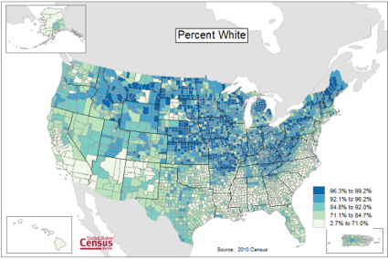
Figure 1. Heat map, USA population by county and percent ethnicity compared to white, graph from census.gov
Note 1: Technically, Figure 1 is an example of a Choropleth Map.
Figure 2 shows gene expression results from a pilot study we did on metal exposure in cultured rat lung cells compared to cells without metal exposure (i.e., the control group). Genes were selected because of their role in the epithelial-mesenchyme transition, EMT. The color scale is typical for such studies: green represents down-regulation, red indicates up-regulation compared to the controls. Black used to show no difference between treatment and control cells.
Figure 2. Heat map, gene expression in cultured rat lung cells exposed to metals
Heat maps are good at directing the viewer to areas of strong association between variables, or in the case of comparisons, to draw strong inferences about the association. However, their chief limitations include gradations between colors; like pie charts, it is difficult to interpret the importance of slight changes in color, and the very use of heat map colors does not imply statistical significance (Chapter 8). Some color palettes are poor choices for viewers who may be color blind. A good source about colors is available in the Graphs section of Cookbook for R.
R and heat maps
Lots of specialized packages will do cluster to heat map. Functions include heatmap, heatmap2, heatmap.plus, NeatMap. We’ll step through how to make a heat map with another pilot study data from our lab.
heatmap(). Here’s another heat map, percent DNA in tail from Alkaline Comet Assay (Figure 3). The same cultured cell line, a rat immortalized Type 2-like alveolar lung cell line L2 cells, were grown in media containing witch-hazel tea, a dilute copper solution, or both witch-hazel tea and copper (unpublished data). The hypothesis was that there would be greater DNA damage in cells exposed to copper compared to cells in hazel tea or a combination of copper and hazel tea. Witch hazel is reputed to have antioxidant properties (Pietta et al 1998). A random sample of 10 cells were sampled from each treatment (between 30 and 60 cells counted for each treatment). Within each treatment values were placed in ascending order, so “Cell 1” corresponds to the lowest value for a measured cell in each treatment.
#data arranged in unstacked worksheet
data <- as.matrix(hazelCuUnstack)

#check the import
head(data)

         Copper       Hazel HazelCopper]
[1,] 0.02404672 0.007185706 0.02663191
[2,] 0.06711479 0.027020958 0.03181153
[3,] 0.12196060 0.037725842 0.03743693
[4,] 0.13308991 0.044762867 0.03851548
[5,] 0.13344032 0.045809398 0.18787608
[6,] 0.17537831 0.060942269 0.19494708

#make the heat map
heatmap(data)
Figure 3. A simple heat map generated by heatmap() function, all default options.
The heatmap() function first runs a cluster analysis to group the cells by columns and rows — so similar cells are grouped together. The row and column dendrograms are default; your data are rearranged by the clustering procedure. To generate the heatmap without the dendrograms, add the following to the R code.
heatmap(data, Rowv = NA, Colv = NA)
ggplot2 and aes(). Not straight forward, but ggplot2 (and therefore the Rcmdr plug-in KMggplot2) can be used. The aes function is part of the “aesthetic mapping” approach (Wickham 2010). The example below takes the same data and introduces use of a custom color palette, brewer.pal. Uses geom_tile, but geom_raster can also be used.
library(RColorBrewer)
#Explore the color profiles available at http://colorbrewer2.org/#type=sequential&scheme=BuGn&n=3
?brewer.pal
hm1.colors <- colorRampPalette(rev(brewer.pal(9, 'RdYlGn')), space='Lab')
#the data set
hazelCu <- read.table("hazelCu.txt", header=TRUE, sep="t", na.strings="NA", dec=".", strip.white=TRUE)
#Confirm the import
head(hazelCu)

Cell Treatment TailPerc
1 1 C 0.02404672
2 2 C 0.06711479
3 3 C 0.12196060
4 4 C 0.13308991
5 5 C 0.13344032
6 6 C 0.17537831

#convert cell number to factor.
hazelCu <- within(hazelCu, {
Cell <- as.factor(Cell)
})

ggplot(hazelCu,aes(x=Treatment,y=Cell,fill=TailPerc)) + geom_tile() + coord_equal() +
scale_fill_gradientn(colours = hm1.colors(100))
Figure 4. ggplot() and aes() functions used to generate a heat map. Colors from brewer.pal
The color scheme used in Figure 3 is common in gene expression studies: green is negative, cooler, while red is positive, hotter.
Questions
- What are three advantages of heat map for communicating data.
- What are three disadvantages of heat map for communicating data.
- What color pallet is considered “color-friendly” for accessible visualization?
Quiz Chapter 4.9
Heat maps
Chapter 4 contents
4.8 – Ternary plots
Introduction
Ternary plots are used to show composition of a mixture of three components. For example, simple soil composition analysis, a ternary plot is used to display the relative proportions of sand, clay, and silt in a soil sample (eg, Shepard’s diagram). The R package soiltexture contains a number of routines for soil analysis, including generating ternary plots. The package also includes a simple graphical user interface, soiltexture_gui().
Consider a soil sample by a sedimentation procedure (“jar test”). From the image at Clemson Cooperative Extension Home and Garden Information Center page, we get
Table 1. Jar test results from image at Clemson Cooperative Extension.
| CLAY | SILT | SAND | Z |
| 8.3 | 25 | 66.6 |
in percent. Z is used to add an additional variable to plot (eg, TT_plot()), like soild organic carbon or pH.
Follow the prompts offered by the GUI and we get Figure 1.
Figure 1. Example of Shepard’s plot with data from Clemson Cooperative Extension using R soiltexture package.
With only one sample, the plot is over kill — The soil is mostly sandy with some silt and very little clay.
To interpret the point on the ternary soil texture diagram:
- Start at the plotted black point near the lower left portion of the triangle.
- Read the sand percentage first:
- Follow lines parallel to the left side of the triangle down toward the bottom axis.
- The point aligns near 67% sand.
- Read the silt percentage:
- Follow lines parallel to the left-bottom side toward the right axis.
- The point corresponds to about 25% silt.
- Read the **clay percentage**:
- Follow horizontal lines toward the left axis.
- The point lies near 8% clay.
Additional fields where ternary plots are common include atmospheric greenhouse gas emissions, CO2 – N2 – O2, from a submarine source Daskalopoulou et al (2002), land cover distribution: urban, agriculture, undeveloped (USGS).
In population genetics, de Finetti diagram is used to display three ratio variables that, together, sum to one. For example, display frequency of the three genotypes of a one gene, two allele system in a population. Download the package Ternary from the R mirror. From the Ternary package, we can get a blank plot by simply calling the function TernaryPlot(). R returns the blank plot to the Graphics window (Fig 2).
Figure 2. Blank Graphics window with initial ternary plot.
The basic ternary plot is shown in Figure 1. Running from one corner to another you can see how the frequencies range from 0 to 100%. While we can use the Ternary package, other packages allow you to make ternary plots too, including HardyWeinberg. This package includes several useful tests of the Hardy Weinberg model for population genetics data, so we’ll use that package.
Our example will use the HWTernaryPlot function in the HardyWeinberg package. Before proceeding with the example, download and install the package.
A nice site on ternary plots in Microsoft Excel (24 steps!) is provided at chemostratigraphy.com. Instructions also worked for LibreOffice Calc (pers. obs.). Take a look at www.ternaryplot.com for a really nice online plot builder.
Example. Recall your basic population genetics, for a locus with 2 alleles with frequency p and q in the population, and given Hardy-Weinberg assumptions apply (e.g., no evolution!), then expected genotype frequencies are given by expanding (p + q)2 = 1.
Consider a population genetics example using Skittles (Fig 3).
Figure 3. A few Skittles® candies.
For several bags, count the greens (p) and the oranges (q). Data for 17 mini bags reported Table 2.
Table 2. Counts of green and orange Skittles from 17 mini bags.
| Bag | GREEN | ORANGE |
|---|---|---|
| bag1 | 4 | 2 |
| bag2 | 8 | 2 |
| bag3 | 3 | 3 |
| bag4 | 3 | 4 |
| bag5 | 5 | 7 |
| bag6 | 5 | 1 |
| bag7 | 13 | 5 |
| bag8 | 4 | 2 |
| bag9 | 6 | 3 |
| bag10 | 3 | 2 |
| bag11 | 5 | 4 |
| bag12 | 9 | 9 |
| bag13 | 0 | 2 |
| bag14 | 7 | 3 |
| bag15 | 5 | 4 |
| bag16 | 6 | 2 |
| bag17 | 2 | 3 |
Next, we calculate the genotype frequencies from our counts. For example, for bag1, p = 4/6 and q = 2/6. We can imagine a diploids at the locus: GG, GO, and OO, with frequencies p2, 2pq, and q2. The frequencies for the three genotypes are shown in Table 2.
Table 3. Genotype frequencies for our hypothetical population of Skittle diploid critters.
| Bag | p^2 | 2pq | q^2 |
|---|---|---|---|
| bag1 | 0.44 | 0.44 | 0.11 |
| bag2 | 0.64 | 0.32 | 0.04 |
| bag3 | 0.25 | 0.5 | 0.25 |
| bag4 | 0.18 | 0.49 | 0.33 |
| bag5 | 0.17 | 0.49 | 0.34 |
| bag6 | 0.69 | 0.28 | 0.03 |
| bag7 | 0.52 | 0.4 | 0.08 |
| bag8 | 0.44 | 0.44 | 0.11 |
| bag9 | 0.44 | 0.44 | 0.11 |
| bag10 | 0.36 | 0.48 | 0.16 |
| bag11 | 0.31 | 0.49 | 0.2 |
| bag12 | 0.25 | 0.5 | 0.25 |
| bag13 | 0 | 0 | 1 |
| bag14 | 0.49 | 0.42 | 0.09 |
| bag15 | 0.31 | 0.49 | 0.2 |
| bag16 | 0.56 | 0.38 | 0.06 |
| bag17 | 0.16 | 0.48 | 0.36 |
For the plot, the HWTernaryPlot function expects counts, not frequencies of three genotypes of a gene in a population, with genotype frequency that sums to one. Table 3 shows calculated genotype data, assuming 20 Skittle diploid critters per bag.
Table 4. Expected genotype counts.
| Bag | GG | GO | OO |
|---|---|---|---|
| bag1 | 9 | 9 | 2 |
| bag2 | 13 | 6 | 1 |
| bag3 | 5 | 10 | 5 |
| bag4 | 4 | 10 | 7 |
| bag5 | 3 | 10 | 7 |
| bag6 | 14 | 6 | 1 |
| bag7 | 10 | 8 | 2 |
| bag8 | 9 | 9 | 2 |
| bag9 | 9 | 9 | 2 |
| bag10 | 7 | 10 | 3 |
| bag11 | 6 | 10 | 4 |
| bag12 | 5 | 10 | 5 |
| bag13 | 0 | 0 | 20 |
| bag14 | 10 | 8 | 2 |
| bag15 | 6 | 10 | 4 |
| bag16 | 11 | 8 | 1 |
| bag17 | 3 | 10 | 7 |
Example
Create an R data.frame called skittles from Table 4. Because HWTernaryPlot requires input only of the genotype data, remove the first column
dSkittles <- subset(skittles, select = -c(Bag) )
require(HardyWeinberg)
#Create a Ternaryplot
HWTernaryPlot(dLactose,100,pch=19, cex=2, region=1,hwcurve=TRUE, curvecols=c("red", "green"), vbounds=FALSE, vertex.cex=2, verbose=TRUE)
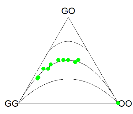
Figure 4. Ternary plot of our Skittle critter data.
What do we have? The function plots three convex curved lines. The green points are the heterozygote (GO) frequencies. They all fall on the middle line, as expected, because I had used HW to calculate frequency of the heterozygotes. If any population had numbers of observed heterozygotes different from expected values, then the population point would be represented by a red point and it would fall in one of the regions above or below the curved lines.
Question
- Repeat the Skittles example, but replace with counts for purple (p) and red (q) candies (scroll down to data below, or click here).
- Optional: A more realistic example would be to draw 2 candies from Skittles bag and record the counts (e,g, how many purple+ purple, purple+red, red+red pairs drawn), then make Ternary plots on the observed and not the expected frequencies.
- Genetic example. The ternary plot is useful for displaying population genetic frequency data. For example, ability to digest lactose, i.e., lactase persistence, is in part due to genotype at SNP rs4988235 (Enattah et al 2002). Genotypes CC tend to be lactose intolerant, genotypes CT and TT are lactose tolerant. I gathered allele frequencies from the ALFA: Allele Frequency Aggregator for several human populations, calculated genotype frequencies assuming Hardy-Weinberg equilibrium. I also created results for a hypothetical population “Madeup.” (Scroll down to data below, or click here). Enter the data into R as a dataframe, eg,
data.SNP, copy R code from this page, make the necessary changes, and recreate the plot shown in Figure 5.- What do you conclude about the heterozygotes in Madeup population?
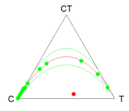
Figure 5. rs4988235 genotype frequencies, data.SNP.
- Add a new row of data to your rs4988235 data set,
data.SNP. CC= 4, CT = 10, TT = 6. The data were derived from frequencies reported in Figure 2, Baffour-Awuah et al 2016 (PMC4308731). To add a new row, modify the code below
data.SNP <- rbind(data.SNP, “PMC4308731” = c(4, 10, 6))
Create another ternary plot, and address whether or not this new data set shows heterozygotes in agreement with Hardy Weinberg assumptions.
Quiz Chapter 4.8
Ternary plots
Data sets
Skittles Data
| Bag | GREEN | ORANGE | RED | PURPLE |
|---|---|---|---|---|
| bag1 | 4 | 2 | 3 | 3 |
| bag2 | 8 | 2 | 4 | 8 |
| bag3 | 3 | 3 | 4 | 2 |
| bag4 | 3 | 4 | 1 | 2 |
| bag5 | 5 | 7 | 6 | 7 |
| bag6 | 5 | 1 | 2 | 3 |
| bag7 | 13 | 5 | 5 | 5 |
| bag8 | 4 | 2 | 5 | 2 |
| bag9 | 6 | 3 | 4 | 4 |
| bag10 | 3 | 2 | 5 | 3 |
| bag11 | 5 | 4 | 2 | 3 |
| bag12 | 9 | 9 | 6 | 8 |
| bag13 | 0 | 2 | 5 | 2 |
| bag14 | 7 | 3 | 6 | 7 |
| bag15 | 5 | 4 | 1 | 3 |
| bag16 | 6 | 2 | 4 | 2 |
| bag17 | 2 | 3 | 1 | 4 |
SNP Data
| Population | C | CT | T |
|---|---|---|---|
| Mambila | 99 | 1 | 0 |
| Ben Amir | 99 | 1 | 0 |
| Zaramo | 100 | 0 | 0 |
| Bedouin | 95 | 5 | 0 |
| Druze | 93 | 7 | 0 |
| Kuwaiti | 86 | 13 | 1 |
| Dutch | 12 | 45 | 43 |
| Finns | 3 | 29 | 68 |
| Swedes | 1 | 13 | 87 |
| Bengali | 87 | 13 | 1 |
| Naga | 100 | 0 | 0 |
| Mala | 88 | 12 | 0 |
| Han | 100 | 0 | 0 |
| Japanese | 100 | 0 | 0 |
| Koreans | 100 | 0 | 0 |
| Cheyene | 93 | 7 | 0 |
| Pima | 98 | 2 | 0 |
| Maya | 90 | 10 | 0 |
| Brazilian | 50 | 42 | 9 |
| Chilean | 60 | 35 | 5 |
| Colombian | 81 | 18 | 1 |
| Madeup | 40 | 5 | 55 |