11.3 – Factors influencing statistical power
Introduction
Components of an experimental design that may influence statistical power include:
- α (probability of committing a Type I error).
As the probability of a Type I error increases, the probability of a Type II error decreases. Therefore, as α gets bigger, power gets decreases. - σ, the variance in the population
Statistical power decreases as variability increases. - Effect size
The effect size is a measure of the differences between two or more groups considered biologically important; its difficult to have lots of power to detect very small differences. - Sample size
As n increases, power increases
Size of alpha (Type I error)
When we introduced the idea of Type I error, alpha, it followed a story about Challenger, the space shuttle that disintegrated after failure of O-rings allowed hot gasses to cross joints in the rockets. If we adopt a Type I error rate of 5% in our rocket designs, then failure is expected at one in twenty launches. That rate clearly is unacceptable, so the logical extension of this thinking would be to decrease the Type I error rate. Unfortunately, this comes at the expense of increasing our risk of Type II error. Thus, decreasing Type I error decreases statistical power.
Variance
If the range of values for individuals in the samples are great, then it should not be surprising that the power to distinguish between sample means from the groups will be low. Conversely, if the variance for a sample is small, then the precision of the estimated sample mean will increase, and, therefore, the power will increase.
Effect size
Effect size deserves some more comments. If we are thinking cause/effect, then we are asking whether or not our independent variable explains a lot of variation in the response (dependent) variable. If there is a strong link between the independent and dependent variable, then the effect size will be large and small numbers of observations will be needed.
There are various ways to estimate effect size, but the simplest is a variation of the t-test (Cohen’s d).

The formula would be different for ANOVA (involves the mean squares), but you get the idea. By convention, an effect size of about 0.2 would be “small,” 0.5 would be “medium,” and an effect size greater than 0.8 would be “large.”
Sample size
This is the area of course where the experimenter has control. We can choose how many individuals are assigned to treatment groups. The Central Limit Theorem basically states that you can use the normal distribution to predict how likely an individual observation is in relation to a sample mean even if the sample distribution is not normally distributed. The larger the number of individuals in the sample from a population, the more confidence we have about making this assumption. Translation: sample size directly impacts standard error of the calculated statistic. Recall our equation for the standard error of the mean.
Alternatives to Cohen’s d
Glass’s g
Hedges’ gu
Keselman and colleagues’ dj
estimators based on trimmed mean and Winsorized variances.
Questions
- The Central limit Theorem can be invoked when we have large samples of observations. In this subchapter we state that increase sample size increases statistical power. Discuss and contrast these two characteristics of large sample size on statistical inference.
- How many samples are enough? Some statistical textbooks will cite a rule of 30. With respect to factors that affect statistical power, discuss the limitations of adopting such a rule to design an experiment.
Quiz Chapter 11.3
Factors influencing statistical power
Chapter 11 contents
- Introduction
- What is Statistical Power?
- Prospective and retrospective power
- Factors influencing statistical power
- Two sample effect size
- Power analysis in R
- References and suggested readings
11.2 – Prospective and retrospective power
Introduction
Statistical power is defined as p = 1 – β. The power of a test is the probability of rejecting a Null Hypothesis when it is false. There is a relationship between Type I error and Type II error. We want β to be Large BUT β is generally not known when we are performing the statistical test. We do know that α is inversely related to β. The smaller the α value we use to Reject the Null Hypothesis the MORE likely we will accept a FALSE Null Hypothesis. If we make α very small (one in a billion) then there would be a very HIGH chance of accepting α Null Hypothesis when it is false (β is high). Note that this is the same discussion that we had about sensitivity of an assay test and the specificity of that assay. If we increase sensitivity of the assay such that we approach 100% detection of the true positives will be detected, we necessarily will increase the number of false positives. The BEST way to reduce both Type I and Type II statistical errors is to INCREASE the sample size!
Power of any statistical test (Z test, T-test, one-way ANOVA…) can be determined BEFORE the experiment is done and data are gathered or AFTER an experiment is completed (Cohen 1992). For now, here’s our first real taste of experimental design — we can evaluate how we can make an experiment to test a particular hypothesis.
Prospective power analysis
Good experimental design should include considerations of power. The design will determine the size of the effect your experiment will be able to detect and the probability of correctly rejecting the null hypothesis. In large part, this will involve decisions of sample size and ways to reduce error variance. Moreover, one needs to decide ahead of time, just how large of an effect does the experiment need to detect??? A one-gram change in body mass before and after a diet treatment is of no concern whatsoever if your study subjects are African elephants, but may be a very large effect for a study of shrews!
Retrospective power analysis
Power analysis can also be done after a test has been conducted and the null hypothesis failed to be rejected. One interpretation that might follow from a retrospective power analysis is that, if the study had low power, the lack of statistical significance could be viewed merely the result of low sample size. However, as forcefully argued Hoenig and Heisey (2001) (see also Colegrave and Ruxton 2003), retrospective or posthoc power tests provide no more information than does the p-value and therefore are redundant. At worse, retrospective power analysis can be misleading as to how well it predicts true power, ie, biologically meaningful differences between different treatment groups (Zhang et al., 2019).
Prospective power is more than effect size between groups
Large effect size, ie, large differences between groups, is not necessarily evidence of important biological differences. The concept of power has limits (Hoenig and Heisey 2001 Yuan and Maxwell 2005). On the other hand, small effect sizes can be important differences, especially if the treatment is difficult or expensive. We work through this conclusion with an example, but emphasize here that providing confidence intervals for the effect size (Colegrave and Ruxton 2003). Suppose the null hypothesis was not rejected from a two sample independent t-test conducted on the test of differences in plant height between two samples of `ohi’a found at different elevations. Was there really no difference or was the sample size in the study simply too small to detect the real and important difference between the samples? By conducting a power analysis, one can determine if a slight increase in sample size would have yielded a statistically significant difference, or it may suggest that the effect size is small enough not to warrant further attention.
R code
Three options for conducting power analysis in R are provided in section 11.5
Questions
- Assuming that a study was done by randomly sampling from a population, and the the primary outcome is found not statistically different with p-value 0.13 between placebo and treatment groups, what can be gained made from a retrospective power analysis?
Quiz Chapter 11.2
Prospective and retrospective power
Chapter 11 contents
- Introduction
- What is Statistical Power?
- Prospective and retrospective power
- Factors influencing statistical power
- Two sample effect size
- Power analysis in R
- References and suggested readings
11.1 – What is Statistical Power?
Introduction
Simply put, the power of a statistical test asks the question: do we have enough data to warrant a scientific conclusion, not just a statistical inference. From the NHST approach to statistics, we define two conditions in our analyses, a null hypothesis, HO, and the alternative hypothesis, HA. By now you should have a working definition of HO and HA (Chapter 8.1). For the two-sided case (Chapter 8.4), HO would be no statistical difference between two sample means, whereas for HA, there was a difference between two sample means. Similarly, for one-sided cases, HO would be one sample mean greater (less) than or equal to the second sample mean, whereas for HA, one sample mean is less (greater) than the second mean. Together, these two hypotheses cover all possible outcomes of our experiment!
However, when conducting an experiment to test the null hypothesis four, not two outcomes are possible with respect to “truth” (Table 1), which we introduced first in our Risk analysis chapter and again when we introduced statistical inference.
Table 1. Possible outcomes of an experiment
| In the population, Ho was really… | |||
| True | False | ||
| Inference: | Fail to reject Ho | Correct decision
p = 1 – α |
Type II error
p = β |
| Reject Ho | Type I error
p = α |
Correct decision
p = 1 – β |
|
We introduced false positives and false negatives in our discussion of risk analysis, and now generalize these concepts to outcomes of any experiment.
(1) We do not reject the null hypothesis, we state that we are 95% (P = 1 – α) confident that we’ve made the correct decision, and in fact, that is the true situation (“correct decision”). As before this is a true positive.
For example, mean acetylsalicylic acid concentration in a sample of 200 mg, brand-name aspirin tablets really is the same as generic aspirin.
(2) We reject the null hypothesis, we state there is a 5% chance that we could be wrong (P = 1 – β), and in fact, that is the true situation (“correct decision”). As before this is a true negative.
For example, ephedrine really does raise heart rates in people who have taken the stimulant compared to those who have taken a placebo.
Two additional possible outcomes to an experiment
The other two possible outcomes are not desirable but may occur because we are making inferences about populations from limited information (we conduct tests on samples) and because of random chance influencing our measure.
(3) We do not reject the null hypothesis, but in fact, there was a true difference between the two groups and we have therefore committed a Type II error. As before this is a false negative.
(4) We reject the null hypothesis, but in fact, there was no actual difference between the two groups and we have therefore committed a Type I error. As before this is a false positive.
What can we do about these two possible undesirable outcomes?
We set our Type I error rate α, and, therefore our Type II error rate β before we conduct any tests, and these error rates cover the possibility that we may incorrectly conclude that the null hypothesis is false (α), or we may incorrectly conclude that the null hypothesis is true (β). When might these events happen?
The power of a statistical test is the probability that the test will reject the null hypothesis when the alternative hypothesis is true.
A type I error is committed, by chance alone, when our sample is accidentally obtained from the tail of the distribution, thus our sample appears to be different from the population… Below, we have a possible case that, by chance alone, we could be getting all of our subjects from one end of the distribution (Fig 1).
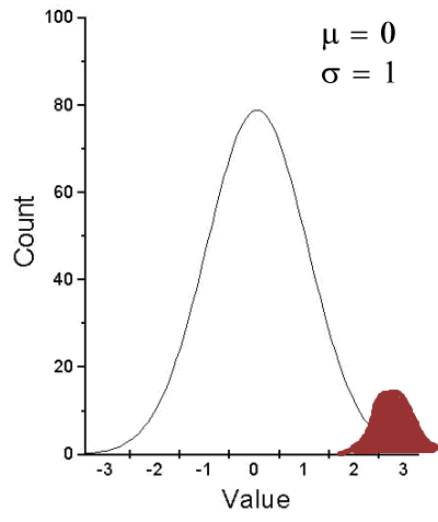
Figure 1. Population sampling from tail of distribution.
We would likely conclude that our sample mean is different (greater) than the population mean.
A type II error is committed, by chance alone, when our sample is between two different population distributions. The implication for our study is drawn in Figure 2. Instead of our sampling drawn from one population, we may have drawn between two very different populations.
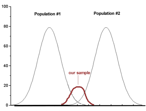
Figure 2. Without us knowing, our sample may come from the extremes of two separate populations.
How did we end up with “the wrong” sample? Recall from our first discussions about Experimental Design how we distinguished between random and haphazard sampling. The key concept was that a program of recruitment of subjects (eg, how to get a sample) must be conducted in such a way that each member of the population has an equal chance of being included in the study. Only then can we be sure that extrinsic factors (things that influence our outcome but are not under our control nor do we study them) are spread over all groups, thus canceling out.
Why do we say we are 95% confident in our estimate (or conclusions)?
(1) Because we can never be 100% certain that by chance alone we haven’t gotten a biased sample (all it takes is a few subjects in some cases to “throw off” our results).
(2) For parametric tests, at least, we assume that we are sampling from a normal population.
Thus, in statistics, we need an additional concept. Not only do we need to know the probability of when we will be wrong (α, β), but we also want to know the probability of when we will be correct when we use a particular statistical test. This latter concept is defined as the power of a test as the probability of correctly rejecting Ho when it is false. Conducting a power analysis before starting the experiment can help answer basic experimental design questions like, how many subjects (experimental units) should my project include? What approximate differences, if any might I expect among the subjects? (Eng 2003; Cohen 1992)
Put another way, power is the likelihood of identifying a significant (important) effect (difference) when one exists. Formally, statistical power is defined as the probability, p = 1 – β, and it is the subject of this chapter.
Questions
- Be able to define and distinguish statistical power and statistical inference.
Quiz Chapter 11.1
What is statistical power
Chapter 11 contents
10.3 – Paired t-test
Introduction
Good experiments include controls. Interested in a new treatment for weight loss? Define a control group to compare the weight loss by a group using the new product. In many cases, the best control is the individual.
Consider now a basic experimental design, the randomized crossover trial (Fig 1), introduced in Chapter 2.4.

Figure 1. A two group Randomized Crossover Trial.
Subjects randomly selected from population of interest, then again once recruited into one of two treatment arms: arm 1, subjects first receive the experimental treatment, then some time later the subjects receive the control treatment; arm 2, subjects first receive the control treatment, then some time later the subjects receive the experimental treatment. Note the difference between this paired or repeated measures design and the independent sample design (see Chapter 10.1). Repeated measures designs have many advantages; we discuss them further in Chapter 14.6. At the start, repeated measures designs have greater statistical power compared to cross-sectional (independent) sample designs.
Many experiments are designed so that subjects receive all treatments and responses are gauged against the initial values recorded on the subjects. Repeated measures statistical tests, like the paired t-test, are needed however to analyze the data. These types of statistical procedures are similar to the two sample independent t-test that we discussed earlier.
However, there is an important difference between these two types of statistical procedures. For the two independent sample t-test the samples are unpaired: we observed one variable on some individuals assigned to two different groups. These groups might be
- Two locations where we measure plants or animals
- A treatment (or experimental) group with a control group.
- Expression of cytokeratin genes (eg, ΔΔCT, fold-change) from breast cancer patients compared to healthy donor subjects (Andergassen et al 2016).
The point is that samples in one group are not the same samples in the second group.
In the paired t-test we have two groups but the observations in these two groups are paired. Paired means that there is some relationship between one observation in the first sample and one observation in the second sample (every observation in one sample must be paired with one observation in another sample).
For example, weight change in humans before and after a change in diet could be performed as a paired analysis. Each subject’s weight before the diet was “paired” with the same subject’s weight after the diet.
Another example comes from genetics. Siblings or Monozygotic twins or clones, strains or varieties of plants or animals can be Paired in an experiment.
- You can give one of the twins a particular diet, or the plant or animal clones or strains can be raised in a particular environment (nutrient)
- The other twin or plant or animal clone or variety can serve as a type of control by providing a normal diet or normal environment.
Another example is a study of environmental pollution on cancer rates in many different communities.
- The researchers selects pairs of communities with similar characteristics for many socioeconomic factors.
- Each pair of communities differed with respect to the proximity to a known source of pollution: one of the pair was close to a source of pollution and one of the pair was far from a source of pollution.
The purpose of pairing in this example is to attempt to “control” for all the socioeconomic factors that might contribute to cancer but they did not want to directly measure. These other factors should be similar for each member of the pair.
Example: How repeatable is human running performance?
The subheading is misleading — we leave “repeatability” or, do individuals perform consistently to another time (see Chapter 12.3 – Fixed effects, random effects, and agreement). Here, we focus on a different question — we test whether mean performance differs across repeated trials. This may seem a subtle difference, but consistency asks the question if performance, whether it is answering questions on an exam or running times for a race, is stable across trials. Testing the means of first and second trials asks a different question: we test for a trend in performance, which may reflect learning.
Here’s an example in which a measure was taken twice for the same individuals. The data are running speed or pace during 5K race held annually on Oahu for a selected sample of female runners with repeat race times (20 – 29 years old). The race was run annually on Oahu, and the data reported are the pace for the first race and the second race, which occurred a year later (Jamba Juice – Banana Man Chase, Ala Moana Beach Park, data extracted from source, https://timelinehawaii.com).
Table 1. 5K pace times (kph) for 15 women (20 – 29 years)
| ID | First race | Second race |
|---|---|---|
| 1 | 15.28 | 15.61 |
| 2 | 11.22 | 11.19 |
| 3 | 8.80 | 9.14 |
| 4 | 8.88 | 5.46 |
| 5 | 9.81 | 10.50 |
| 6 | 6.12 | 5.69 |
| 7 | 8.31 | 8.71 |
| 8 | 6.26 | 7.42 |
| 9 | 17.16 | 16.41 |
| 10 | 16.23 | 15.82 |
| 11 | 5.90 | 7.12 |
| 12 | 8.31 | 10.48 |
| 13 | 5.93 | 8.64 |
| 14 | 10.54 | 5.99 |
| 15 | 9.53 | 8.69 |
Note 1: We’ll return to this data set in Chapter 15.3
Load the data into R as an unstacked data set. Data available at end of this page or click here.
Begin with description and exploration of the data. Start with histograms to get a sense of the sample distributions (hint: we’re looking to see if the data looks like it could come from a normal distribution, see Chapter 13.3 Assumptions) (Fig 2).
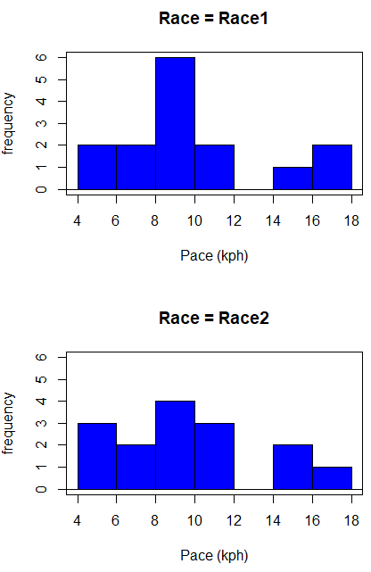
Figure 2. Histograms shows the distribution of 5K running times of 15 women who ran the race twice.
R code (stacked data set, then used defaults R Commander to make the histogram, then modified the code and submitted modified code to make Fig 1)
with(stackExCh10.3, Hist(obs, groups=Race, scale="frequency", breaks="Sturges", col="blue",
xlab="Time (min)", ylab="Frequency")))
Conclusion? The histograms don’t look normally distributed so we keep this in mind as we proceed. (See Chapter 13 – Assumptions of parametric tests for additional information about assumptions.)
A box plot comparing the first and second pace times (Fig 3).
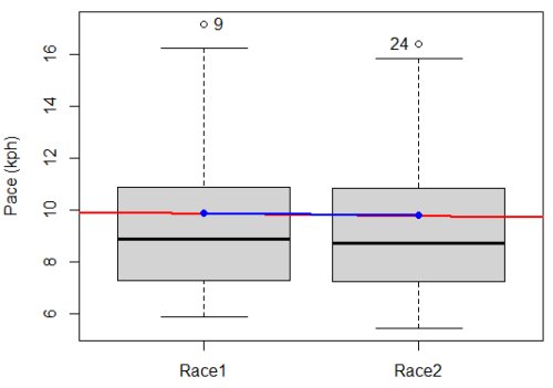
Figure 3. Box plot of race speed (kph) for 15 women 5K in two successive years.
I added a trend line (linear regression, see Chapter 17, red line) and connected the averages (blue line) for visual emphasis — no differences between the means — but note that one wouldn’t do this as part of an analysis (see Chapter 4 discussion).
R code for Fig 2
Boxplot(obs~Race, data=stackExCh10.3, id=list(method="y"), xlab="", ylab="Pace (kph)") #boxplot was made in Rcmdr
abline(lm(obs ~ as.numeric(Race), data=stackExCh10.3), col="red", lwd=2)
means <- tapply(obs, Race, mean)
points(1:2, means, pch=7, col="blue")
lines(1:2, means, col="blue", lwd=2)
The box plot works to show the median difference, but loses the paired information. A nice package called PairedData has several functions that work well with paired data, for example a profile plot (Fig 4). A profile plot is useful for showing an association between paired data.
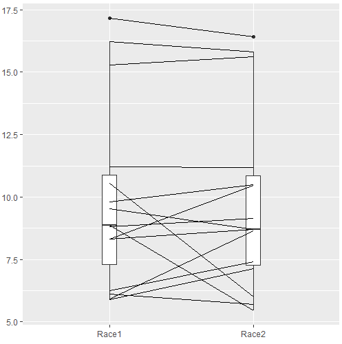
Figure 4. Profile plot, PairedData package.
R commands for Figure 4.
require(PairedData)
attach(example.ch10.3) # remember to attach dataframe so you don't have to call variables like example.ch10.3$Race1
races <- paired(Race1, Race2)
plot(races, type = "profile")
Paired t-test calculation
The paired t-test is a straight-forward extension of the independent sample t-test; the key concept is that the two samples are no longer independent, they are paired. Thus, instead of mean of group 1 minus mean of group two, we test the differences between sample 1 and sample 2 for each paired observation.

- Compute the differences between the Paired Samples (as in tables above)
- Calculate the MEAN difference score,
 : in the previous example = -0.094 kmh
- Calculate the degrees of freedom df = # pairs – 1 = n – 1, where n is the number of pairs
- Calculate the standard error of the mean of d.

where

- Calculate the test statistic for paired data

- Compare to the Critical Value in Table C. 4 (Appendix Table 2)
- Find the Critical Value = t α (2), df
Try as difference instead of paired
Before you answer, take a look at the box plot of the mean difference between the repeat measures of 5K pace for the 15 women (Fig 5).
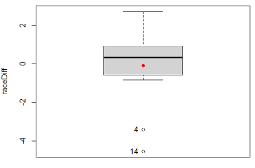
Figure 5. Box plot of differences, Red dotted lines shows the null hypothesis.
Note 2: Figure 5 is appropriate for diagnostics, but not for publication, per our discussions in Chapter 4.
Create a new variable, raceDiff, equal to Race2 minus Race1. Then, use the one sample T-test on raceDiff. I’ll leave you to complete the work (Question 2).
R code
t.test(Race1, Race2, paired = TRUE, alternative = "two.sided")
R output
Paired t-test

data: Race.1 and Race.2
t = 0.19389, df = 14, p-value = 0.849
alternative hypothesis: true difference in means is not equal to 0
95 percent confidence interval:
-0.9491017 1.1377521
sample estimates:
mean of the differences
0.09432517
Rcmdr, paired t-test
Rcmdr: Statistics → Means → Paired t-test…
Note: your two groups must be in two different columns (unstacked!) to run this version of the test.
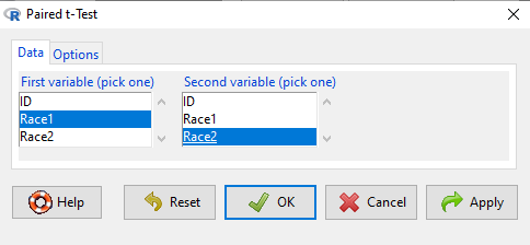
Figure 6. R Commander Paired t-test menu, Rcmdr version 2.7.
After selecting the variables, set null hypothesis after clicking on Options tab (Fig 6).
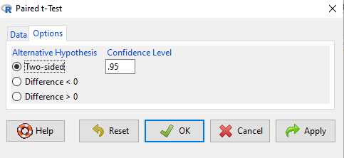
Figure 7. R Commander Paired t-Test options, select null hypothesis.
Click OK to proceed. Results will be the same as the output listed above.
the following text needs to be updated
Interpret the results.
So, what can we conclude about the null hypothesis? Interpret the 95% CI, the T-test statistic, and the P-value.
Do not ignore sample dependence
What if we ignored the repeated measures design and treated the first and second races as independent? The important concept here is to ask, what would have happened if we had done a two independent sample t-test instead?
Let’s run the analysis again, this time incorrectly using the independent sample t-test. We need to manipulate the data set before we do.
Manage your data: Stack the data
This is a good time to share how to Stack data in R. If you look at our active data set, the results of the two trials are in two different columns. In order to run the independent sample t-test we need the data in one column (with a label column).
stackExCh10.3 <- stack(example.ch10.3[, c("Race1","Race2")])
names(stackExCh10.3) <- c("obs", "Race")
Rcmdr: Data → Active data set → Stack variables in data set…
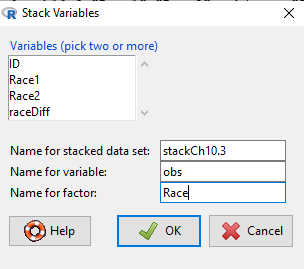
Figure 8. R Commander: Stack worksheet. Select the two variables, Race1 and Race2.
I entered values for name of the new data set, the new variable, and the name for the factor (label) column.
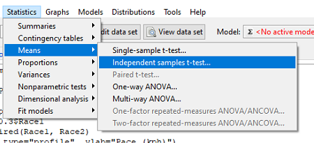
Figure 9. R Commander, select independent sample t-Test …
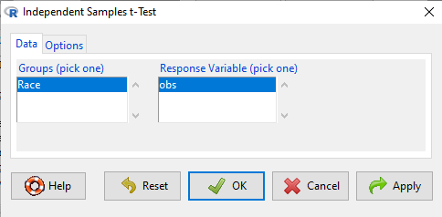
Figure 10. R commander, independent sample t test menu.
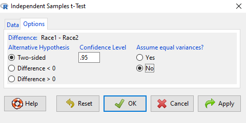
Figure 11. R Commander, select options for independent sample t-Test (assume equal variance).
Here are the results of the independent sample t-test from R.
t.test(obs~Race, alternative='two.sided', conf.level=.95, var.equal=TRUE, + data=stackCh10.3)

Two Sample t-test
data: obs by Race
t = 0.070645, df = 28, p-value = 0.9442
alternative hypothesis: true difference in means is not equal to 0
95 percent confidence interval:
 -2.640719 2.829369
sample estimates:
mean in group Race1 mean in group Race2
 9.886342 9.792017
End R output
In this case, we would have reached the same general conclusion, but the p-values are different. The p-value from the paired t-test was about 0.85 whereas the p-value from the independent sample t-test was higher, nearly 0.95, suggesting little difference between the two trials.
While the general conclusion holds, this time, that there were no statistically significant difference between the means for first and second trials. However, it won’t always work out that way. And besides, if you treated the paired data as independent, you’ve clearly violated one of the assumptions of the test.
Take a look at the degrees of freedom for the two analyses. By ignoring the pairing of samples we gain twice the number of degrees of freedom … that can’t both be right. The way to distinguish between the two is to go back to the experimental units.
Question: What are the sampling units in the case of repeat measures on individuals: the individuals themselves? the pairs of burst speed trials? something else?
it is important to note that the paired t-test is still the best for this situation because it accurately reflects the experiment — individuals were measured twice, therefore the two groups (trial 1 and trial 2) are not independent! Thus, the p-value from the paired t-test correctly reflect our best analyses of the test of the null hypothesis because the correct degrees of freedom were 14 and not 28.
In the case of the independent sample t-test we necessarily make the assumption that the two groups are independent — that is, that they are measured on different sampling units (eg, different individuals or subjects). In statistical terms, that means that you assume that the correlation between trial results is equal to zero. By incorrectly choosing an independent sample test in these repeated measures cases, I would make two null hypotheses: (1) that the means are the same and (2) that the correlation between repeat measures is zero. The problem? The t-test only evaluates the first hypothesis (means).
Questions
- Refer to Figure 6 again and related data set. Were runners faster the second year or the first year running the 5k? What about the points labeled 4 and 14? What was the average difference between first and second races?
- Complete the test of the null hypothesis of no difference between race 1 and race 2 (
raceDiff) with the one sample t-test. Set up a table to compare the test statistic, df, and p-values for results from paired t test, one sample t-test, and independent sample t-test. How do these results compare? - I’ve called the observed value “pace,” but runners would know that pace is actually amount of time per kilometer, not the total time over 5k, which is what I called pace.
- Create a new variable and report average pace for Race1 and Race2.
- Redo the paired analysis, including box plot, on your new variable.
- What is the null hypothesis for your new variable?
- Summarize your results and add to the table you created for question 2.
- Redo the two plots in Figure 2 so that the two histograms are on the sample plot. Instructions and examples were provided in Chapter 4.2.
Quiz Chapter 10.3
Paired t-test
Data set
example.ch10.3 <- read.table(header=TRUE, text = "
ID Race1 Race2
1 15.28 15.61
2 11.22 11.19
3 8.80 9.14
4 8.88 5.46
5 9.81 10.50
6 6.12 5.69
7 8.31 8.71
8 6.26 7.42
9 17.16 16.41
10 16.23 15.82
11 5.90 7.12
12 8.31 10.48
13 5.93 8.64
14 10.54 5.99
15 9.53 8.69
")
Chapter 10 contents
10.2 – Digging deeper into t-test Plus the Welch test
Introduction
We need to spend some more time with the independent sample t-test; by tearing it apart, we can learn about how parametric tests work in general.
Our assumptions for the independent sample t-test are like the one-sample t-test the data must be continuous and normally distributed (one of our standard assumptions for parametric tests, see Chapter 13). The formula is very similar to the one-sample t-test, except that now we have two sample means and the formula for the standard error (SE) has also changed.

We see that the test statistic t is large if the numerator is large compared to the denominator. Large values of t will be evidence in favor of rejecting the null hypothesis.
The numerator is straightforward: we subtract one sample mean from the other — if there is no difference between the samples, then this difference will be close to zero.
The denominator requires additional discussion. What is it called? It is the pooled standard error of the mean (pooled SEM). Provided the assumption of equal variances holds — an additional standard assumptions for parametric tests, see Chapter 13 — then sample variances estimate the population variance and we can use this information to our advantage to best test the hypothesis about the sample means. In other words, we don’t have to lose a degree of freedom to account for differences in variability for the two groups (see Welch test). More degrees of freedom means more statistical power to test the null hypothesis and at the same time, more confidence that the test is performing to its best.
Lets break down the pooled standard error of the mean in order to see how the assumption of equal variances affects the t-test. We assume that 
Recall that

Now we want a “pooled SE” that is the pooled standard error for both samples. The variance of the difference between the means can be written as
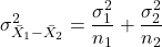
First we need to calculate the pooled variance. where v1 and v2 are degrees of freedom for sample one and sample two, respectively.
Note 1This is just simply a combined formula of the sample variance.
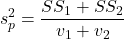
What is SS? The sum of squares , where SS1 and SS2 refer to sum of squares for each of the two groups.
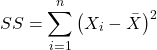
You should recognize SS from your definition of the sample variance, Chapter 3.3.
And the standard error for the difference between two means can now be written as So the 2-sample t-test can be written to reflect the pooled sample standard error of the difference between two sample means. We can see how unequal sample size is accommodated by the t-test.
Conducting the test by hand follows the same form as the one-sample t-test. Find the degrees of freedom (DF), but now for each sample.
Finally we evaluate with the critical value in Table (Appendix, Table of Student’s t distribution) and compare the t test statistic against the critical value with the appropriate degrees of freedom.
Because this is the t-test, again, we are assuming that the variances are the same between the two populations (homoscedasticity) and this allows us to pool the variance. As it turns out, the T-test is not overly sensitive to other deviations from the assumptions, but if the variances are in fact different, then the standard formula may yield incorrect Type I error rates compared to stated probability level (α).
However, it would be poor statistical choice to use a test where there are alternatives. This is why in part that R (Rcmdr) sets as the default for the t-test that variances are unequal! In fact, R does not do a t-test unless you change the default to assume equal variances, which, as we now know, is the t-test.
Welch test
What to do when assumptions to t-test are not met? Many options have been proposed, and Welch’s approximate t is a good alternative to the two-sample t-test — it would be appropriate if the normal assumption still held.
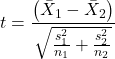
The degrees of freedom for the Welch’s test are now
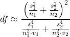
Note 2: The Welch test removes the pooled estimate of the standard error, replaces with both variance estimates directly.
As a default option, R and Rcmdr uses a variation of Welch’s test when you select to do the t-test without making the assumption of equal variance (Fig 1).
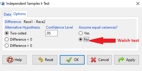
Figure 1. Screenshot Rcmdr t-test options. Default is “No” for Assume equal variances, ie, the Welch test.
The Welch test is not a nonparametric test, it is a different formulation of the t-test.
Justification for beginning with t-test
It’s unlikely that you will need the t-test in today’s research climate. Data sets are large, experiments are complex with multiple variables and samples. Why do we have to consider the t-test, and then a separate test in the case for unequal sample size? I view it as a teaching moment. It makes the general point that ALL statistical tests make assumptions about how the calculations are done and as to the nature of the data set.
This is our first experience with what to do if there is a violation of an assumption of parametric tests (see Chapter 13). Here, the assumption is that the two groups have equal sample size. When they do not, the standard t-test tends to biased estimates. On the other hand, if the assumptions are met, the standard test is the best test because it has more power to do what we intended — that is, it is best at the actual test of the null hypothesis! Take heart — this point is not always appreciated even by scientists (cf. Fagerland 2012).
Note 3: Expert advice will differ here, but you can always calculate the test statistic, even if the assumptions do not hold. The problem, the concern is with the interpretation.
Let’s us approach the problem of violation of assumptions in a couple of ways as an introduction to how, in general, to approach choice of statistical tests.
- Power of a test. Much current statistical research focuses on learning about how a particular statistical test works when assumptions are violated. Thus, in addition to learning what tests are designed to do, we need to consider the effects of violations of assumptions on the performance of the test (namely, is the Type I error at the stated alpha level?). This is a matter of statistical power; power of a test reflects how able the test is to get you the correct result even if assumptions are violated. Often tests perform well if sample sizes are large despite violation of assumptions. We mention without proving that the 2-sample T-test is robust to violations of normality assumption, to requirement for equal sample size, and even to unequal variances. But good experimental design attempts to meet the assumptions because the test does better!
- Alternate forms of some tests are available to handle some aspects of test violations. For example, the simple 2-sample T-test can be modified to accommodate different variances (Welch’s formula). Or you must find a different test (eg, nonparametric tests).
In conclusion, all tests begin with consideration of the assumptions. In some cases we can test our assumptions. For example, we learned about testing the assumption of normal distributions of sample data. We can also test the assumption of equal variances.
Questions
- Consider a clinical trial in which resting blood pressure is recorded on hypertensive subjects at the start of the trial, then 6 weeks after subjects have received daily supplements of flaxseed. Thus, for each subject there are two measures of blood pressure, BEFORE and AFTER.
- Write the null hypothesis
- Write the alternative hypothesis
- Justify why or why not the hypothesis should be two tailed. Explain why or why not an independent sample t-test may be used to compare groups.
Quiz Chapter 10.2
Digging deeper into t-test Plus the Welch test
Chapter 10 contents
- Introduction
- Compare two independent sample means
- Digging deeper into t-test Plus the Welch test
- Paired t-test
- References and suggested reading
10.1 – Compare two independent sample means
Introduction
We introduced the concept of comparing a sample statistic (mean) against a population parameter (Chapter 6.7, Normal deviate) or one-sample t-test against a specified mean (eg, from published data or from theory, Chapter 8.5).
Consider now a basic experimental design, the randomized control trial, or RCT (Fig 1), introduced in Chapter 2.4.
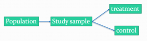
Figure 1. A two group Randomized Control Trial.
Subjects randomly selected from population of interest, then again — random assignment — once recruited into one of two treatment groups. Importantly, subjects belong to one treatment arm only: no subject simultaneously receives the treatment and the control. This is in contrast to the paired design, in which subjects receive both treatments (see Chapter 10.3).
In inferential statistics about an experiment, we are more likely trying to test if sample means are different. For example
- two species grown in common garden, do they differ in growth rate?
- human subjects given a new treatment have better outcomes compare to those receiving a control treatment (eg, placebo).
The equivalent null hypothesis is that two samples are pulled from the same population. We write the null hypothesis as

and the corresponding alternative hypothesis, HA, then must be

Question: Is this a one tailed or two-tailed hypothesis?
Answer: Two-tailed (review Chapter 8.4)
Note 1: In this day and age, there’s really no compelling reason to learn the t-test. First, it is just a special case of the one-way ANOVA, therefore, it’s a special case of the general linear model. Struggling to learn R commands? Well, one solution would be just to learn the general linear model approach — the R function lm() (OK — don’t get too excited — lm() has many options and details). Second, few experiments or observational studies are likely to have only two groups; thus, the temptation to carry out a series of t-tests, taking all groups two at a time, or “pairwise,” while tempting, actually violates a whole bunch of basic statistical rules (discussed in Chapter 12.1). It will also make statisticians go crazy when they see it. That said, if your experiment has but two groups, then by all means, the t-test is a choice. The t-test is also a statistical test that you have likely already used before so we present the discussion here to build on what you may already have learned. We also present the independent t-test as a vehicle.
Worked example
We introduce the two-sample t-test, or better, the independent sample t-test.

where the numerator is the difference between the two sample means and the denominator is the standard error of the differences between the two groups standard errors. The formula for
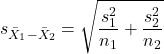
The choice of independent sample over two-sample is best because it emphasizes that the two groups (the two samples), must be comprise of independent sampling units. This is a pretty straight-forward requirement; you have randomly assigned twenty individuals to two groups, a control group (n = 10) and a treatment group (n = 10). Individuals are either in the control group or they are in the treatment group — they cannot simultaneously appear in both groups.
We will work our way through this test by example. For starters, let’s use the same lizard dataset (see Example data set, below), four body mass recordings (grams) each for house geckos (Hemidactylus frenatus, Fig 2) and the Carolina anole (Anolis carolensis, Fig 3), two of many lizard species introduced to Hawaiʻi.

Figure 2. Male Hemidactylus frenatus, central Oahu, M. Dohm.

Figure 3. Male Anolis carolinensis, ʻAkaka Falls, Big Island of Hawaiʻi, M. Dohm.
Example data set
Geckos: 3.186, 2.427, 4.031, 1.995

Anoles: 5.515, 5.659, 6.739, 3.184
Question: How would you go about creating a data frame with the values in long form (stacked worksheet), including a label variable and the body mass?
Note 2: The independent sample t-test in Rcmdr requires a stacked worksheet and not in unstacked worksheet two columns implied by the above pseudo-code. If you need help with worksheet format, then see Part07 in Mike’s Workbook for Biostatistics.
Answer: At the R prompt, type
Geckos <- c(3.186, 2.427, 4.031, 1.995); Anoles = c(5.515, 5.659, 6.739, 3.184) #create two vectors
bmass <- c(Geckos, Anoles)    #combine the two vectors into a single vector holding all of the body mass records
species <- c("gecko", "gecko", "gecko", "gecko", "anole", "anole", "anole", "anole")   #create your label variable
lizards <- data.frame(species, bmass)  #create your data frame
lizards   #print your data frame  species bmass
1   gecko 3.186
2   gecko 2.427
3   gecko 4.031
4   gecko 1.995
5   anole 5.515
6   anole 5.659
7   anole 6.739
8   anole 3.184
Note also that you can enter data into the Data editor by creating the data frame first then adding values. To edit the data frame “lizards” type fix(lizards) at the R prompt, then close the data frame when you have added or changed values as needed.
As always, begin with an exploration of the data, including a graph (Fig 4).
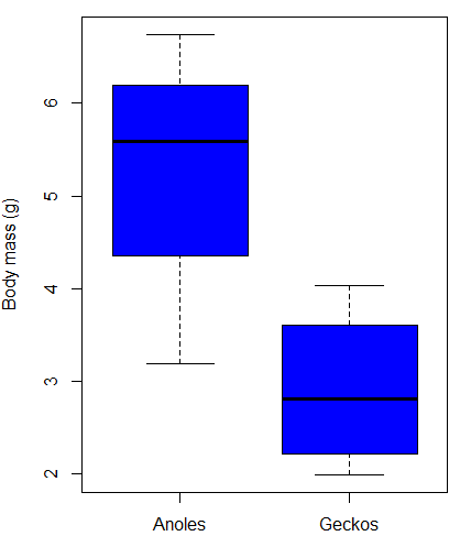
Figure 4. Box plot of lizard body mass.
We can see already that there’s greater spread of data for the Anoles compared to the Geckos, but the median values differ. Small sample sizes can be a problem for analyses as we can only have reduced confidence in our conclusions. However, we press on for the sake of demonstration.
Let’s test the null hypothesis, H0, ie, the two species of lizards have the same mean body mass.
Rcmdr: Statistics → Means → Independent-samples t-test…
In this next image I posted the Rcmdr menu popup for the Independent Samples t-test (Fig 5). Later versions of Rcmdr split the settings for this command into two tabs; the first tab allows for the selection of the variables and setting the hypotheses whereas the second tab, labeled Options, permits additional choices. The default selections need your attention: to actually conduct the t-test you need to answer “No” to the question, “Assume equal variance?” (Fig 6).
Figure 5. Rcmdr menu for Independent sample t-test.
Select the Options tab (Fig 6) to select null hypothesis and to select the t-test and not the Welch-test (which is the default, ie, No to the prompt “Assume equal variances?”).
Figure 6. Rcmdr Options menu for Independent sample t-test.
Let’s look at the results and break down the parts of the test.
t.test(Body.mass~Lizard, alternative='two.sided', conf.level=.95,
+ var.equal=TRUE, data=lizards)

Two Sample t-test

data: Body.mass by Lizard
t = 2.7117, df = 6, p-value = 0.03503
alternative hypothesis: true difference in means is not equal to 0
95 percent confidence interval:
0.2308685 4.4981315
sample estimates:
mean in group Anolis mean in group Gecko
5.27425 2.90975
Consider the R session output above and answer the following questions.
Questions for the worked example
- Which lizard group had the greater mean value, Anolis or Gecko?
- What are the assumptions necessary for you to use the independent sample t-test?
- What does “two-sided” mean?
- What was the null hypothesis?
- Was this a one-tailed or two-tailed test of the null hypothesis?
- What is the value of the test statistic?
- How many degrees of freedom?
- What is the critical value for this test?
- What is the value of the lower limit of the 95% confidence interval?
- What is the value of the lower limit of the 99% confidence interval?
- True or False. If the null hypothesis is accepted, then zero is a value included in the 95% confidence interval.
- Do you accept the null hypothesis? Explain your selection.
Try another example
DNA damage, changes in the chemical structure of nucleotide bases or breakage of the DNA chains, occurs in cells under many circumstances. The comet assay, or single-cell gel electrophoresis, is one method for visualizing and measuring DNA strand breaks in cells. Exposed cells are mixed with a low-melting temperature agarose and placed onto a microscope slide. The cells are then lysed with an alkaline detergent and high salts. When current is applied across the slide, undamaged DNA remains in the nucleus, whereas damaged DNA extends towards the anode to form a comet-like tail, with imaging assisted by including a fluorescent dye like Sybr-Green. Examples of comets are shown below (Fig 7).
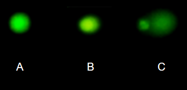
Figure 7. Comet examples. A Intact cell, no DNA damage, B Cell with some DNA damage, a slight tail to the right is evident, C Cell with significant DNA damage, a large tail is evident. M. Dohm.
In an experiment, immortalized lung epithelial cells were exposed to dilute copper solutions for 30 minutes then washed with PBS. The comet assay was applied to these cells and for comparison, to cells without copper exposure but otherwise treated the same way (controls). The data are available at the bottom of this page (scroll down or click here).
Again, you should begin all analyses with an exploration of the data, including a graph (Fig 8).
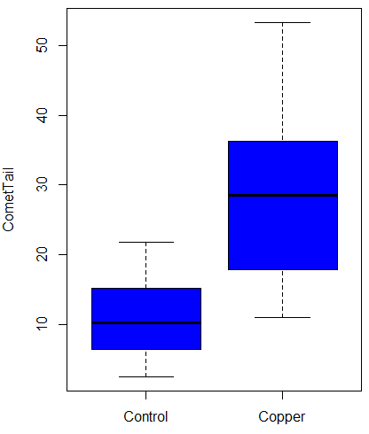
Figure 8. Boxplot of comet tail lengths for cells with and without (control) exposure to copper in the cell medium for 30 minutes.
Let’s look at the R output for the t-test analysis.
    Two Sample t-test

data:  CometTail by Treatment
t = -5.8502, df = 38, p-value = 9.139e-07
alternative hypothesis: true difference in means is not equal to 0
95 percent confidence interval:
 -22.39865 -10.88213
sample estimates:
mean in group Control  mean in group Copper
             11.14533              27.78571
Consider the R session output above and answer the following questions.
Questions for Comet assay data set
- Which cell group had the greater mean value, Copper-exposed or Control-exposed cells?
- What are the assumptions necessary for you to use the independent sample t-test?
- What does “two-sided” mean?
- What was the null hypothesis?
- Was this a one-tailed or two-tailed test of the null hypothesis?
- What is the value of the test statistic?
- How many degrees of freedom?
- What is the critical value for this test?
- What is the value of the lower limit of the 95% confidence interval?
- What is the value of the lower limit of the 99% confidence interval?
- True or False. If the null hypothesis is accepted, then zero is a value included in the 95% confidence interval.
- Do you accept the null hypothesis? Explain your selection.
T test from summary statistics
In some cases you may only have to summary statistics for data, eg, the means and the standard deviations. We can use the equations of the t test to write a simple formula, where the user provides the known means, standard deviations, and sample size. For example, create a simple function with readline for user input.
myTtest <- function() {
   mnx <- as.numeric(readline(prompt="Enter mean of x: "))
   stdevx <- as.numeric(readline(prompt="Enter sd of x: "))
   nx <- as.numeric(readline(prompt="Enter n of x: "))
   mny <- as.numeric(readline(prompt="Enter mean of y: "))
   stdevy <- as.numeric(readline("Enter sd of y: "))
   ny <- as.numeric(readline(prompt="Enter n of y: "))
   myTvalue <- abs(((mnx-mny)-0)/sqrt(((stdevx^2)/nx)+(stdevy^2)/ny))
   myDF <- as.integer(nx+ny-2)
   myPvalue <- pt(myTvalue,myDF,lower.tail=FALSE)*2
   myResults <- c(myTvalue, myDF, myPvalue)
   report <- c("T-test: ", "df: ", "two-tailed p-value: ")
   cat(sprintf("%s %3.3f, ", report, myResults))
}
then run the function by typing myTest() at the R prompt and entering the means, standard deviations, and sample size when prompted.
myTtest()
Enter mean of x: 2.91
Enter sd of x: .895
Enter n of x: 4
Enter mean of y: 5.27
Enter sd of y: 1.497
Enter n of y: 4
T-test: 2.706, df: 6.000, two-tailed p-value: 0.035
P-values from confidence intervals
While we expect certain reporting criteria for published, it is not uncommon that one or more elements are missing. For example, while means plus or minus standard deviations for two groups may be reported, the confidence interval of the difference may not be reported, or, an inexact p-value is reported like “< 0.05,” but we “need” an exact p-value for our meta-analysis. A little math, and these missing statistics can be calculated.
We can use the lizard study as an example; while all of the expected elements were reported, including the p-value (0.03503), let’s say the p value was reported as “statistically significant at p < 0.05.”
We need
lower and upper confidence intervals: 0.2309 and 4.498, respectively.
critical value from t distribution, df = 6 (2 tailed, therefore 0.05/2). A little R code we have:

the standard error, which can be calculated as 
and then the p-value, 
which is pretty close to the result from R (p = 0.03503). The difference is likely due to the small sample size.
Questions
- Don’t forget to work through the Questions for the Comet tail data set (scroll up or click here).
- Microsoft Excel, LibreOffice Calc, and Google sheets spreadsheet software all include t-test functions and return the p-value. Consider two variables big (100, 110, 120, 100, 110, 210, 200) and small (0,1,1,2,0,1,0). (Note — these two groups are obviously very different, calculating a t-test on their difference is silly, just for this question.) If formatting is set to the default two decimal places for Number cell category, the p-value will return as “0.00.” How should you report the p-value in this case?
Quiz Chapter 10.1
Compare two independent sample means
Comet assay data set
| Treatment | CometTail |
| Control | 17.856139 |
| Control | 16.52125 |
| Control | 14.925449 |
| Control | 14.029174 |
| Control | 13.332945 |
| Control | 8.811185 |
| Control | 14.701654 |
| Control | 9.261025 |
| Control | 21.779311 |
| Control | 6.180284 |
| Control | 9.201752 |
| Control | 5.54472 |
| Control | 6.717885 |
| Control | 2.625092 |
| Control | 7.191583 |
| Control | 5.392866 |
| Control | 11.284813 |
| Control | 15.441254 |
| Control | 17.857176 |
| Control | 4.250956 |
| Copper | 53.214287 |
| Copper | 38.92857 |
| Copper | 18.928572 |
| Copper | 30 |
| Copper | 28.928572 |
| Copper | 15.357142 |
| Copper | 17.857143 |
| Copper | 17.5 |
| Copper | 21.071428 |
| Copper | 29.285715 |
| Copper | 28.214285 |
| Copper | 16.785715 |
| Copper | 21.071428 |
| Copper | 37.5 |
| Copper | 38.214287 |
| Copper | 17.857143 |
| Copper | 29.642857 |
| Copper | 11.071428 |
| Copper | 35 |
| Copper | 49.285713 |
Chapter 10 contents
- Introduction
- Compare two independent sample means
- Digging deeper into t-test Plus the Welch test
- Paired t-test
- References and suggested reading
9.6 – McNemar’s test
Introduction
There are a number of scenarios in which subjects are paired or matched as part of the experimental design in order to control for confounding variables — a matched pair case-control. Subjects may be matched by age, or other criteria, or the observations are repeat measures of the same subjects (eg, left hand vs. right hand). One member of each pair is then randomly assigned to a treatment, the remaining pair member then assigned to the other treatment group. This scenario should remind you of our standard contingency table problem, but instead of a random collection of subjects assigned to treatments, the data are paired nominal. Thus, paired means that experimental (sampling) units are not independent, which if ignored violates an assumption required to employ the  test. We use McNemar’s test instead.
The possible results of such a design include just two outcomes: the pairs have the same outcome (agree, concordant) or the pairs have different outcomes (disagree, discordant).
McNemar’s solution was to consider only the discordant pairs. Consider two kinds of tests or assays for a condition, and the doctor receives the results of both tests. Our familiar two-by-two table results, and in this scenario may be called a confusion table — after all, there is truth and agreement along the diagonal including cells a and d are agreement between the two methods, whereas the off diagonal cells c and b are “confusion,” the two methods disagree.
Table 1. The familiar 2X2 table, now used to display agreement between two different testing procedures.
| Test 2 | ||||
| Positive | Negative | Row total | ||
| Test 1 | Positive | a | b | a+b |
| Negative | c | d | c+d | |
| Column total | a+c | b+d | n | |
Null hypothesis is that marginal proportions are equal

then McNemar’s test is given by
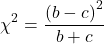
and the test has one degree of freedom.
If one of the cells is low, then a continuity correction would be applied (Edwards 1948, cited in Fagerland et al 2013). With this correction the equation becomes
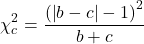
If either b or c is small, then the McNemar’s test statistic does not approximate a distribution very well, so there is a binomial version that you would use (Cochran’s Q test); used in cases where there are three or more matched sets and is common in meta-analysis (Kulinskaya and Dollinger 2015).
R code
Example data: Approval ratings for President Trump at two important markers during the Covid-19 pandemic: April 2020, deaths passed 10,000 persons in the US; in October 2020, it was reported that President Trump tested positive for SAR-COV2 and was admitted to Walter Reed National Military Medical Center (admitted 3 Oct, released 5 Oct). Surveys were conducted by YouGov (April, sponsored by The Economist; October, sponsored by Yahoo News; data extracted from How Americans View Biden’s Response To The Coronavirus Crisis)
Table 2. Approval ratings for President Trump at two important markers during the Covid-19 pandemic, data from YouGov survey.
| Approve | Disapprove | |
| April survey | 720 | 705 |
| October survey | 645 | 812 |
Enter the data as a matrix (note this would be a general approach for the contingency table problems, too, instead of entering via Rcmdr menu). The discordant pairs are b = 645 and c = 705
covid19 <- matrix(c(720, 645, 705, 812), nrow = 2, dimnames = list("April survey" = c("Approve", "Disapprove"), "October survey" = c("Approve", "Disapprove")))

 covid19
                      October survey
April survey       Approve   Disapprove
         Approve       720          705
      Disapprove       645          812
Uncorrected
mcnemar.test(covid19, correct=FALSE)

McNemar's Chi-squared test

data: covid19
McNemar's chi-squared = 2.6667, df = 1, p-value = 0.1025
Correction applied
mcnemar.test(covid19, correct=TRUE)

McNemar's Chi-squared test with continuity correction

data: covid19
McNemar's chi-squared = 2.5785, df = 1, p-value = 0.1083
Conclusions?
No change in approval ratings. The correction for small sample size had little effect on p-value, unsurprisingly, given that the surveys included 1500 (April) and 1504 (October) persons.
Unconditional paired tests
McNemar’s solution considers only the discordant pairs; it’s a conditional test. The downside of these tests is that the concordant pairs are not considered. Thus, by in effect tossing out some portion of the experimental results, it shouldn’t surprise you that the statistical power of the test is reduced (see Chapter 11). Thus, McNemar’s test may no longer be the best choice. Alternative unconditional tests have been proposed, and the mid-P alternative shows promise (Routledge 1994; Fagerland et al 2013). The mid-P value is calculated as the standard p-value for a test statistic minus one half the difference between the standard p-value and the next lowest possible p-value. McNemar’s mid-p test is available in package contingencytables. Try with example data set in Fagerland et al 2013 (Table 1).
#create a 2x2 matrix
bentur <- rbind(c(1, 1), c(7, 12))
First run McNemar’s test without correction for small sample size.
mcnemar.test(bentur, correct=FALSE)
R output follows
McNemar's Chi-squared test

data: bentur
McNemar's chi-squared = 4.5, df = 1, p-value = 0.03389
Next, run McNemar’s test with correction for small sample size.
mcnemar.test(bentur, correct=TRUE)
R output follows
McNemar's Chi-squared test with continuity correction

data: bentur
McNemar's chi-squared = 3.125, df = 1, p-value = 0.0771
Last, run min-p version of McNemar’s test.
McNemar_midP_test_paired_2x2(bentur)
R output
[1] The McNemar mid-P test: P = 0.039063
See also mcnemarExactDP function in exact2x2 package. Without explanation, here’s the R code and results
mcnemarExactDP(n = sum(bentur), m= bentur[1,2] + bentur[2,1], x = bentur[1,2])

      Exact McNemar Test (with central confidence intervals)

data: n=sum(bentur) m=bentur[1, 2] + bentur[2, 1] x=bentur[1, 2]
n = 21, m = 8, x = 1, p-value = 0.07031
alternative hypothesis: true difference in proportions is not equal to 0
95 percent confidence interval:
 -0.54549962 0.02044939
sample estimates:
       x/n    (m-x)/n  difference
0.04761905 0.33333333 -0.28571429
Alternatively, use wrapper function mnemar.exact().
mcnemar.exact(bentur)
R output
Exact McNemar test (with central confidence intervals)

data: bentur
b = 1, c = 7, p-value = 0.07031
alternative hypothesis: true odds ratio is not equal to 1
95 percent confidence interval:
 0.003169739 1.111975554
sample estimates:
odds ratio
 0.1428571
Note the alternative hypothesis: p-value is two-tailed.
Quiz Chapter 9.6
McNemar's test
Questions
1. Apply McNemar’s test and mid-P exact test to CDC example
| Controls | |||
| Cases | Exposed | Not exposed | |
| Exposed | 58 | 89 | |
| Not exposed | 32 | 95 | |
Chapter 9 contents
9.5 – Fisher exact test
Introduction
We mentioned that chi-square tests for contingency tables are fine as long as two conditions are met. These are the assumptions of a test.
- No cell should have expected values less than 5%.
- The test performs poorly at DF = 1 because we are approximating an infinite distribution with an exact test.
You will note that any time you have a 2X2 table, the second condition is always an issue because 2X2 tables have DF=1. Thus, in biomedical research, it is common to have an experiment that may be appropriate for a contingency analysis but the data may suffer from one or both of these limitations. Fisher’s exact test is always an option for these types of problems, but with the advantage that it always returns the exact p-value.
A reminder, the 2×2 table looks like
Table 1. 2×2 table reporting numbers of subjects who have (Yes) or do not have (No) the event.
| Column 1 | Column 2 | ||
| Subjects | Yes | No | |
| Row 1 | Treatment 1 | a | b |
| Row 2 | Treatment 2 | c | d |
where a is the count of Treatment 1 – treated subjects who have the event, b is the count of Treatment 1 – treated subjects who do not have the event, c is the count of Treatment 2 – treated subjects who have the event, d is the count of Treatment 2 – treated subjects who do not have the event. Note the row and column totals:
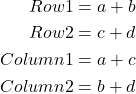
For example, a fairly common, “Gee, that’s curious,” fact is the seven left-handed US Presidents since 1901 (21), is higher than the proportion of left-handers in the general population (about 10%). For comparison, we could ask the same question about Vice Presidents.†
Table 2. U.S. Presidents and Vice-Presidents handedness.
| Subjects | Yes | No |
| Presidents | 7 | 14 |
| Vice presidents | 5 | 20 |
†Seven Vice-Presidents went on to become President, four right-handers, three left-handers.
Ronald A. Fisher came up with a test that is now called “Fisher’s Exact test” that circumvents this problem. It is an extremely useful test to know about because it provides a way to get an exact probability of the outcome compared to all other possible outcomes. Thus, when asked for a possible alternate to the chi-square contingency test for a 2X2 table, you can respond “Fisher’s Exact test.”
Although tedious to calculate by hand, and resource demanding when done by computer because of the multiple factorial expressions, the major advantage of the test is that it does not rely on the assumption that an underlying distribution applies. The Fisher Exact test can be used to calculate the exact probability of the observed outcome (P).
The equation for the Fisher Exact test can be written as
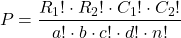
where R stands for row total, C stands for column total, n is the sample size, ! is the factorial, and a, b, c, and d are defined as in Table 1.
How does Fisher’s Exact test work? The data are setup in the usual way for a contingency problem, but now, we calculate the probability for all possible outcomes that we COULD have seen from our experiment, and ask if the actual outcome is unusual (low p-value). The trick is recognizing that you have to keep the totals constrained (note row and column totals stay the same).
Table 3. Original 2X2 contingency table (bold), with the next two more extreme outcomes.
| original data |  |
more extreme | |
next more extreme still | |
| Yes | No | Yes | No | Yes | No |
| 10 | 5 | 11 | 4 | 12 | 3 |
| 4 | 12 | 3 | 13 | 2 | 14 |
 |
 |
 |
I’ve shown just the one-tailed outcomes, so the p-values are for one-tailed tests of hypothesis. The essence of the test is to find all outcomes MORE extreme than the original, in one direction. The one-tailed P-value then is the sum of all probabilities from those more extreme tables of outcomes.
To get the two-tailed probability, remember that you multiply the one-tailed probability by two. More accurate methods are also available (Agresti 1992).
Calculation of Fisher’s test involves using all possible combinations and factorials. Rcmdr has Fisher’s 2X2 built in via the Contingency table and as part of some Rcmdr plugins (eg, RcmdrPlugin.EBM, the Evidence Based Medicine plugin). Here we illustrate Fisher Exact test from the context menu in the main Statistics menu.
Alternatively, there are many web sites out there that provide an online calculator for Fisher’s Exact test. Here’s a link to one such calculator on GraphPad’s web site, cookies must be enabled to run this calculator).
To get the Fisher Exact test, your data must already be summarized into a 2X2 table, in which case you can use R Commander via the Contingency tables… menu selection (Fig 1).
Table 4. 2X2 table smokers vs vitamin use.
| Smoker: No | Smoker: Yes | |
| Vitamin use: No | 14 | 26 |
| Vitamin use: Yes | 19 | 15 |
With the data summarized as in Table 4, we can proceed directly via R Commander to analyze the contingency table, either by Chi-square test of Fisher exact test. First, bring up menu to enter the data (Fig 1):
Rcmdr: Statistics → Contingency tables… → Enter and analyze two-way table…
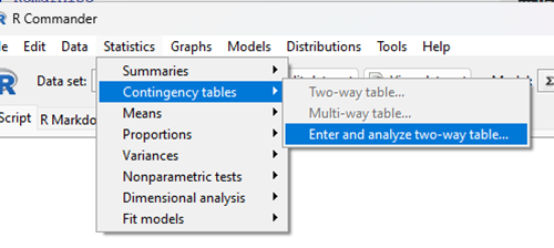
Figure 1. Screenshot Rcmdr menu, Contingency tables.
The image of the R worksheet below contains two columns: Smoker (No, Yes) and Vitamin use (No, Yes). Complete the form (Fig 2).
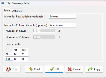
Figure 2. Screenshot Rcmdr menu, Enter Two-Way Table.
Alternatively, if the original data are available, do not tally the counts, let R do the work for you. The worksheet would be stacked like so (Table 5).
Table 5. Portion of subject and row entries in stacked worksheet for smokers vs vitamin use.
| Subject | Vitamin.use | Smoking |
| 1 | No | No |
| 2 | No | No |
| 3 | No | No |
| 4 | No | No |
| 5 | No | No |
| . | . | . |
| 71 | Yes | Yes |
| 72 | Yes | Yes |
| 73 | Yes | Yes |
| 74 | Yes | Yes |
And from the R Commander menu select as before
Rcmdr: Statistics → Contingency tables… → Two way table … (Fig 3).
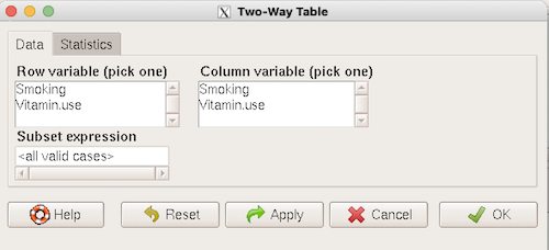
Figure 3. Screenshot Rcmdr two-way table menu, load the data from stacked worksheet.
Data is now ready.
R code
To carry out contingency table analysis on the entered data (Fig 2 or Fig 3), select the Statistics option tab (Fig 4, green arrow).
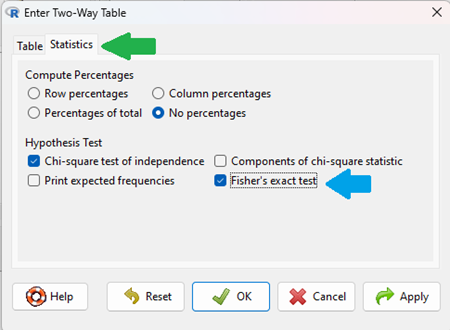
Figure 4. Screenshot Rcmdr menu Statistics option. Select Chi-square test of independence, Fisher’s exact test, or both.
Check the box next to the Fisher’s exact test (Fig 4, blue arrow).
Click OK, and here is the R output.
> fisher.test(.Table)
Fisher's Exact Test for Count Data

data: .Table
p-value = 0.1008
alternative hypothesis: true odds ratio is not equal to 1
95 percent confidence interval:
0.1496417 1.1985775
sample estimates:
odds ratio
0.4302094
We accepted the defaults Is this a one or two-tailed test of hypothesis?
What can we conclude about the null hypothesis? Do we accept or reject?
Want to know what the “odds ratio” is? Follow the link to the next subchapter.
When to use the Fisher Exact Test?
Here’s the take-home message: the Fisher exact test is an alternate and better choice over the contingency table chi-square for 2X2 tables if one or more of the cells has expected values less than 5%. It is also appropriate for cases in which you have only 1 degree of freedom (as do all 2X2 tables!), but it doesn’t make sense if each cell has more than 5% expected values (the calculation is too tedious), but rather, apply the Yate’s correction. As the sample sizes get larger, the different methods converge to virtually identical answers.
Some examples.
Is there an association between final grades and attendance on a randomly selected day?
Table 6. First 2X2 scenario.
| cc | Yes | No |
| Letter grade A | 2 | 3 |
| Other letter grade | 1 | 6 |
Table 7. Second 2X2 scenario.
| cc | Yes | No |
| Letter grade A | 5 | 6 |
| Other letter grade | 2 | 12 |
Table 8. Third 2X2 scenario.
| cc | Yes | No |
| Letter grade A | 10 | 12 |
| Other letter grade | 4 | 24 |
Code hints for tests with direct 2X2 entry with matrix() are
grades.Table <- matrix(c(2,3,1,6), 2, 2, byrow=TRUE)
Chi-square test of independence
chisq.test(grades.Table, correct=FALSE)
Fisher Exact test
fisher.test(grades.Table, alternative = "greater")
Questions
1. Apply Fisher exact test on the four contingency tables (a – d) introduced in section 9.3, question 2. Make note of the p-value from Fisher exact test and from analyses used to complete question 2. Note any trends. (Hint: make sure you are testing the same null hypothesis.)
(a)
| Yes | No | |
| A | 18 | 6 |
| B | 3 | 8 |
(b)
| Yes | No | |
| A | 10 | 12 |
| B | 3 | 14 |
(c)
| Yes | No | |
| A | 5 | 12 |
| B | 12 | 18 |
(d)
| Yes | No | |
| A | 8 | 12 |
| B | 3 | 3 |
Quiz Chapter 9.5
Fisher Exact Test
Chapter 9 contents
9.4 – Heterogeneity chi-square tests
Planned comparisons and meta-analysis.
After finding evidence to reject the statistical null hypothesis, it may be appropriate to proceed to test a number of data sets against the same theoretical distribution. Provided these are planned comparisons, part of the experiment and not an exercise in data dredging (Norman 2014), you may proceed to test a series of nested models where groups are combined to make new groups for comparison. This approach is analogous to the post-hoc tests one may conduct after a statistically significant ANOVA (see Chapter 12.4) or when identifying a best-fit regression model (see Chapter 18.4).
Combining groups to make new comparisons — this scenario is consistent with a meta-analysis. A type of systematic review (Greenhalgh 1997, Akobeng 2005), meta-analysis is a statistical method that combines the results from multiple independent studies on the same topic to provide a more precise and robust overall conclusion. By combining studies, the goal is to calculate a pooled estimate as a measure of overall effectiveness of the treatment. Meta-analysis can increase the overall sample size, which improves the study’s ability to detect an effect if one exists. So, how to combine results from different studies ostensibly addressing the same hypothesis? Inevitably, some subjectivity will come into decisions about including or excluding studies — the goal is to identify quality studies, which may have conflicting conclusions and test whether a single conclusion of effectiveness is warranted based on a summary of evidence.
Here we introduce the Cochran’s Q test (Cochran 1954, Hoaglin 2016), aka a special case of the more general heterogeneity chi-square test. The null hypothesis is no significant difference in the proportion of “successes” across all groups being compared — any observed differences between the groups are just due to chance. The test statistic, Q, has a chi-square distribution with  degrees of freedom. A large Q value and small p-value suggest significant heterogeneity of results among the studies.
Note 1. As a reminder, “success” as an outcome category in epidemiology studies can represent any result depending on the study’s objective: survival, recovery, symptom improvement, or prevention of infection. The alternative outcome is generally referred to as “failure” (eg, death, non-recovery, no improvement, infection).
Heterogeneity tests ask whether results from combined studies are consistent; other tests exist, and are detailed in our special chapter on conducting meta-analysis. For example, I2 or I-squared test provides a measure of how much variation in the combined studies is due to true differences rather than by chance. In short, the I2 test quantifies how much — the percentage — the different studies agree, while the chi-square test returns a p-value that can be used to interpret whether that heterogeneity is statistically significant. We outline the basics of meta-analysis in Chapter 20.15. Other tests include DerSimonian-Laird test and Mandel-Paule test — these use the Q statistic and its distribution to estimate the between-study variance and provide better estimators with small sample size. Between-study variance is used to determine if a fixed-effect or a random-effects model (Chapter 12.3 and Chapter 14.3), is appropriate for the analysis. A random-effects model is used when significant heterogeneity is present (Higgins et al 2009).
Example.
Imagine a scenario where a population geneticist has collected allele (gene) frequency and genotype frequency data on single nucleotide polymorphisms (SNP) for the BRCA1 locus for three USA groups, African Americans, Asian Americans, and European Americans. Data of this kind can be obtained from the SNP database at NCBI (data retrieved 14 & 15 July 2014), and I collated several SNP involving a Cytosine base for Thymine base change (Table 1). The BRCA1 locus is on chromosome 17 and some of the hundreds of mutations found for this gene are associated with high risk of breast and or ovarian cancer (Couch and Weber 1996, Tram et al 2013).
Table 1. SNP of BRCA1 locus
| SNP | Population | n | C/C | C/T | T/T | C | T |
| rs1060915 | African American | 46 | 0.043 | 0.174 | 0,783 | 0.130 | 0.870 |
| Asian American | 48 | 0.083 | 0.625 | 0.375 | 0.396 | 0.604 | |
| European American | 48 | 0.167 | 0.458 | 0.375 | 0.396 | 0.604 | |
| rs3737559 | African American | 40 | 0.043 | 0.174 | 0.783 | 0.130 | 0.870 |
| Asian American | 48 | 0.083 | 0.625 | 0.292 | 0.396 | 0.604 | |
| European American | 48 | 0.167 | 0.458 | 0.375 | 0.396 | 0.604 | |
| rs799917 | African American | 124 | 0.048 | 0.258 | 0.694 | 0.177 | 0.823 |
| Asian American | 90 | 0.467 | 0.444 | 0.089 | 0.689 | 0.311 | |
| European American | 118 | 0.407 | 0.458 | 0.136 | 0.636 | 0.364 |
We may wish to test the combined data set to see if the large data set differs from Hardy Weinberg expectations before proceeding with a series of sample populations. By combining the data sets, we will be able to test whether one genotype is different from exception.
The goal then is to pool the data so that you have a more powerful test of the null hypothesis (remember our general discussion of statistical power and how increasing sample size increases your chances of correctly rejecting the null hypothesis).
For example, in our test of Hardy-Weinberg expectations (Example C), we calculated a test of 7.8955. This test has k – 1 = 3 – 1 = 2 degrees of freedom. At alpha 5%, the critical value was 5.991 We clearly would reject the null hypothesis. But do we reject because of a difference in the aa, ab, or bb genotypes? Simply combine categories. Let’s test the homozygotes (aa and bb) versus the heterozygotes (ab).
Table 2. Worksheet
|
Categories
|
|||
| aa + bb | ab | n | |
|
Observed
|
66 | 34 | 100 |
|
Expected
|
52 | 48 | 100 |
 |
 |
||
With one degree of freedom, we clearly reject the null hypothesis because the critical value at 5% and one degree of freedom is equal to 3.841. To get the p-value, use
pchisq(7.852,df=1,lower.tail=FALSE)
which will return
[1] 0.005076452
Oh, and what was the null hypothesis? That there was an equal number of homozygotes and heterozygotes.
Other tests would be possible here, but the point is that you can dissect an experiment to determine which group is causing you to reject the null original hypothesis. While this is an important tool, you should also consider issues of apriori and aposterori decisions in experiments.
Questions.
1. The SNP rs1799971 (A > G) in the μ-opioid receptor (MOR) is associated with opioid dependency. Allele frequencies for different populations are provided in the table. Global frequency for A at this SNP is 0.188 (therefore frequency of G is 0.812).
| Population | n | A | G |
|---|---|---|---|
| African American | 32510 | 0.97 | 0.03 |
| Central American | 2450 | 0.81 | 0.19 |
| European | 18872 | 0.86 | 0.14 |
| Native American | 1260 | 0.86 | 0.14 |
| Native Hawaiian | 4534 | 0.75 | 0.25 |
| South Asian | 856 | 0.59 | 0.41 |
- Combine the data sets and test whether genotype frequency is different from the reported global exception.
- Test each population separately.
2. A behavioral ecologist studies the effect of three diets (high-protein, high-carbohydrate, and mixed) on the growth rate of juvenile frogs. Before collecting any data, she writes a protocol stating that she will compare only the high-protein vs mixed diet, based on a specific hypothesis about amino acid availability.
After analyzing the data, she also notices that frogs on the high-carbohydrate diet seem smaller, so she performs several additional pairwise comparisons that were not part of her original plan, reporting only the ones that are statistically significant.
Which statement best distinguishes the planned comparison from data dredging (p-hacking)?
A. The planned comparison is valid because it uses a larger sample size, while data dredging uses small samples.
B. The planned comparison was specified ahead of time based on a biological hypothesis, while data dredging involves unplanned tests added after seeing the data to search for significant results.
C. The planned comparison uses ANOVA, while data dredging uses regression.
D. The planned comparison must always produce a significant result, while data dredging never does.
Quiz Chapter 9.4
Heterogeneity chi-square tests
Chapter 9 contents
9.3 – Yates continuity correction
Introduction
Yates continuity correction: Most statistical textbooks at this point will note that critical values in their table (or any chi-square table for that matter) are approximate, but don’t say why. We’ll make the same directive — you may need to make a correction to the for low sample numbers. It’s not a secret, so here’s why.
We need to address a quirk of the test: the chi-square distribution is a continuous function (if you plotted it, all possible values between, say, 4 and 3 are possible). But the calculated statistics we get are discrete. In our HIV-HG co-infection problem from the previous subchapter, we got what appears to be an exact answer for P, but it is actually an approximation.
We’re really not evaluating our test statistic at the alpha levels we set out. This limitation of the goodness of fit statistic can be of some consequence — increases our chance to commit a Type I error — unless we make a slight correction for this discontinuity. The good news is that the does just fine for most df, but we do get concerned with it’s performance at df = 1 and for small samples.
Therefore, the advice is to use a correction if your calculated is close to the critical value for rejection/acceptance of the null hypothesis and you have only one df. Use the Yate’s continuity correction to standard calculation,  .
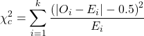
For the 2×2 table (Table 1), we can rewrite Yates correction

Our concern is this: without the correction, Pearson’s test statistic will be biased (eg, the test statistic will be larger than it “really” is), so we’ll end up rejecting the null hypothesis when we shouldn’t (that’s a Type I error). This becomes an issue for us when p-value is close to 5%, the nominal rejection level: what if p-value is 0.051? Or 0.049? How confident are we in concluding accept or reject null hypothesis, respectively?
I gave you three examples of goodness of fit and one contingency table example. You should be able to tell me which of these analyses it would be appropriate to apply to correction.
More about continuity corrections
Yates suggested his correction to Pearson’s back in 1934. Unsurprisingly, new approaches have been suggested (eg, discussion in Agresti 2001). For example, Nicola Serra (Serra 2018; Serra et al 2019) introduced
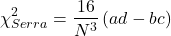
Serra reported favorable performance when sample size was small and the expected value in any cell was 5 or less.
R code
When you submit a 2X2 table with one or more cells less than five, you could elect to use a Fisher exact test, briefly introduced here (see section 9.5 for additional development), or, you may apply the Yates correction. Here’s some code to make this work in R.
Let’s say the problem looks like Table 1.
Table 1. Example 2X2 table with one cell with low frequency.
| Yes | No | |
| A | 8 | 12 |
| B | 3 | 22 |
At the R prompt type the following
library(abind, pos=15)
#abind allows you to combine matrices into single arrays
.Table <- matrix(c(8,12,3,22), 2, 2, byrow=TRUE)
rownames(.Table) <- c('A', 'B')
colnames(.Table) <- c('Yes', 'No') # when you submit, R replies with the following table
.Table  # Counts
 Yes No
A  8 12
B  3 22
Here’s the command; the default is no Yates correction (ie, correct=FALSE); to apply the Yates correction, set correct=TRUE.
.Test <- chisq.test(.Table, correct=TRUE)
Output from R follows
.Test
    Pearson's Chi-squared test with Yates' continuity correction
data:  .Table
X-squared = 3.3224, df = 1, p-value = 0.06834
Compare without the Yates correction
.Test <- chisq.test(.Table, correct=FALSE)
.Test
    Pearson's Chi-squared test
data:  .Table
X-squared = 4.7166, df = 1, p-value = 0.02987
Note that we would reach different conclusions! If we ignored the potential bias of the un-corrected we would be tempted to reject the null hypothesis, when in fact, the better answer is not to reject because Yates-corrected p-value is greater than 5%.
Just to complete the work, what does the Fisher Exact test results look like (see section 9.5)?
fisher.test(.Table)
    Fisher's Exact Test for Count Data
data:  .Table
p-value = 0.04086
alternative hypothesis: true odds ratio is not equal to 1
95 percent confidence interval:
0.9130455 32.8057866
sample estimates:
odds ratio
  4.708908
Which to use? The Fisher exact test is just that, an exact test of the hypothesis. All possible outcomes are evaluated and we interpret the results as likely as p=0.04086 if there is actually no association between the treatment (A vs B) and the outcome (Yes/No) (see section 9.5).
Questions
- With respect to interpreting results from a test for small samples, why use the Yates continuity correction?
- Try your hand at the following four contingency tables (a – d). Calculate the test, with and without the Yates correction. Make note of the p-value from each and note any trends.
(a)
| Yes | No | |
| A | 18 | 6 |
| B | 3 | 8 |
(b)
| Yes | No | |
| A | 10 | 12 |
| B | 3 | 14 |
(c)
| Yes | No | |
| A | 5 | 12 |
| B | 12 | 18 |
(d)
| Yes | No | |
| A | 8 | 12 |
| B | 3 | 3 |
3. Ch09.1, Question 1 provided an example of a count from a small bag of M&Ms. Apply the Yates correction to obtain a better estimate of p-value for the problem. The data were four blue, two brown, one green, three orange, four red, and two yellow candies.
- Construct a table and compare p-values obtained with and without the Yates correction. Note any trend in p-value
Quiz Chapter 9.3
Yates continuity correction