19.2 – Bootstrap sampling
Introduction
Bootstrapping is a general approach to estimation or statistical inference that utilizes random sampling with replacement (Kulesa et al. 2015). In classic frequentist approach, a sample is drawn at random from the population and assumptions about the population distribution are made in order to conduct statistical inference. By resampling with replacement from the sample many times, the bootstrap samples can be viewed as if we drew from the population many times without invoking a theoretical distribution. A clear advantage of the bootstrap is that it allows estimation of confidence intervals without assuming a particular theoretical distribution and thus avoids the burden of repeating the experiment.
Base install of R includes the boot package. The boot package allows R users to work with most functions, and many authors have provided helpful packages. I highlight a couple packages
install packages lmboot, confintr
Example data set, Tadpoles from Chapter 14, copied to end of this page for convenience (scroll down or click here).
Bootstrapped 95% Confidence interval of population mean
Recall classic frequentist (large-sample) approach to confidence interval estimates of mean by R
x = round(mean(Tadpole$Body.mass),2); x
n = length(Tadpole$Body.mass); n
s = sd(Tadpole$Body.mass); s
error = qt(0.975,df=n-1)*(s/sqrt(n)); error
lower_ci = round(x-error,3)
upper_ci = round(x+error,3)
paste("95% CI of ", x, " between:", lower_ci, "&", upper_ci)
Output results are
> n = length(Tadpole$Body.mass); n
[1] 13
> s = sd(Tadpole$Body.mass); s
[1] 0.6366207
> error = qt(0.975,df=n-1)*(s/sqrt(n)); error
[1] 0.384706
> paste("95% CI of ", x, " between:", lower_ci, "&", upper_ci)
[1] "95% CI of 2.41 between: 2.025 & 2.795"
We used the t-distribution because both  the population mean and
 the population standard deviation were unknown. Thus, 95 out of 100 confidence intervals would be expected to include the true value.
Bootstrap equivalent
library(confintr)
ci_mean(Tadpole$Body.mass, type=c("bootstrap"), boot_type=c("stud"), R=999, probs=c(0.025, 0.975), seed=1)
Output results are
Two-sided 95% bootstrap confidence interval for the population mean based on 999 bootstrap replications
and the student method

Sample estimate: 2.412308
Confidence interval:
    2.5%    97.5%
2.075808 2.880144
where stud is short for student t distribution (another common option is the percentile method — replace stud with perc), R = 999 directs the function to resample 999 times. We set seed=1 to initialize the pseudorandom number generator so that if we run the command again, we would get the same result. Any integer number can be used. For example, I set seed = 1 for output below
Confidence interval:
    2.5%    97.5%
2.075808 2.880144
compared to repeated runs without initializing the pseudorandom number generator:
Confidence interval:
    2.5%    97.5%
2.067558 2.934055
and again
Confidence interval:
    2.5%    97.5%
2.067616 2.863158
Note that the classic confidence interval is narrower than the bootstrap estimate, in part because of the small sample size (i.e., not as accurate, does not actually achieve the nominal 95% coverage). Which to use? The sample size was small, just 13 tadpoles. Bootstrap samples were drawn from the original data set, thus it cannot make a small study more robust. The 999 samples can be thought as estimating the sampling distribution. If the assumptions of the t-distribution hold, then the classic approach would be preferred. For the Tadpole data set, Body.mass was approximately normally distributed (Anderson-Darling test = 0.21179, p-value = 0.8163). For cases where assumption of a particular distribution is unwarranted (e.g., what is the appropriate distribution when we compare medians among samples?), bootstrap may be preferred (and for small data sets, percentile bootstrap may be better). To complete the analysis, percentile bootstrap estimate of confidence interval are presented.
The R code
ci_mean(Tadpole$Body.mass, type=c("bootstrap"), boot_type=c("perc"), R=999, probs=c(0.025, 0.975), seed=1)
and the output
Two-sided 95% bootstrap confidence interval for the population mean based on 999 bootstrap replications
and the percent method
Sample estimate: 2.412308
Confidence interval:
    2.5%    97.5%
2.076923 2.749231
In this case, the bootstrap percentile confidence interval is narrower than the frequentist approach.
Model coefficients by bootstrap
R code
Enter the model, then set B, the number of samples with replacement.
myBoot <- residual.boot(VO2~Body.mass, B = 1000, data = Tadpoles)
R returns two values:
bootEstParam, which are the bootstrap parameter estimates. Each column in the matrix lists the values for a coefficient. For this model,bootEstParam$[,1]is the intercept andbootEstParam$[,2]is the slope.origEstParam, a vector with the original parameter estimates for the model coefficients.seed, numerical value for the seed; use seed number to get reproducible results. If you don’t specify the seed, then seed is set to pick any random number.
While you can list the $bootEstParam, not advisable because it will be a list of 1000 numbers (the value set with B)!
Get necessary statistics and plots
#95% CI slope
quantile(myBoot$bootEstParam[,2], probs=c(.025, .975))
R returns
    2.5%    97.5%
335.0000 562.6228
#95% CI intercept
quantile(myBoot$bootEstParam[,1], probs=c(.025, .975))
R returns
     2.5%     97.5%
-881.3893 -310.8209
Slope
#plot the sampling distribution of the slope coefficient
par(mar=c(5,5,5,5)) #setting margins to my preferred values
hist(myBoot$bootEstParam[,2], col="blue", main="Bootstrap Sampling Distribution",
xlab="Slope Estimate")
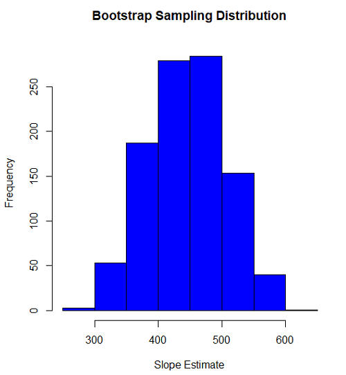
Figure 1. histogram of bootstrap estimates for slope
Intercept
#95% CI intercept
quantile(myBoot$bootEstParam[,1], probs=c(.025, .975))
par(mar=c(5,5,5,5))
hist(myBoot$bootEstParam[,1], col="blue", main="Bootstrap Sampling Distribution",
xlab="Intercept Estimate")
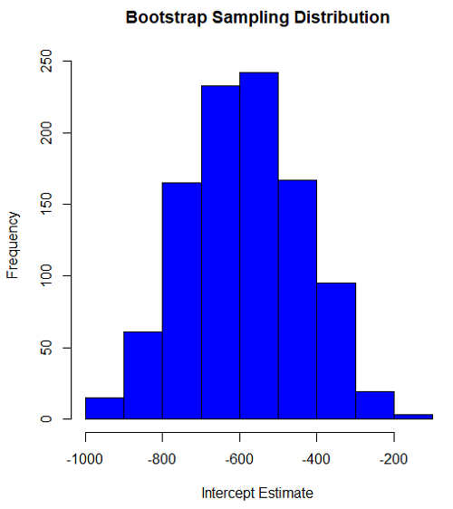
Figure 2. Histogram of bootstrap estimates for intercept.
Questions
edits: pending
Data set used this page (sorted)
| Gosner | Body mass | VO2 |
| I | 1.76 | 109.41 |
| I | 1.88 | 329.06 |
| I | 1.95 | 82.35 |
| I | 2.13 | 198 |
| I | 2.26 | 607.7 |
| II | 2.28 | 362.71 |
| II | 2.35 | 556.6 |
| II | 2.62 | 612.93 |
| II | 2.77 | 514.02 |
| II | 2.97 | 961.01 |
| II | 3.14 | 892.41 |
| II | 3.79 | 976.97 |
| NA | 1.46 | 170.91 |
Chapter 19 contents
- Introduction
- Jackknife sampling
- Bootstrap sampling
- Monte Carlo methods
- Ch19 References and suggested readings
6.4 – Types of probability
Introduction
By probability, we mean a number that quantifies the uncertainty associated with a particular event or outcome. If an outcome is certain to occur, the probability is equal to 1; if an outcome cannot happen, the probability is equal to zero. Most events we talk about in biology have probability somewhere in between.
A basic understanding, or at least an appreciation for probability is important to your education in biostatistics. Simply put, there is no certainty in biology beyond simple expectations like Benjamin Franklin’s famous quip about “death and taxes…”
Discrete probability
You are probably already familiar with discrete probability. For example, what is the probability that a single toss of a fair coin will result in a “heads?” The outcomes of the coin toss are discrete, categorical, either “heads” or “tails.”
Note 1: Obviously, this statement assumes a few things — coin tossed not in a vacuum, for example. We assume a fair coin — equal chance heads or tails. Fair coins have two sides; tossing a coin we expect “heads” or “tails,” but rarely, some coin types may land and come to rest on edge or side (eg, USA nickels). We still consider the coin toss having binary outcomes, by definition, even though a coin may land on edge about one toss in six thousand (Murray and Teare 1993) because the exception is extremely rare. h/t Dr. Jerry Coyne.
And for ten tosses of the coin? And more cogently, what is the probability that you will toss a coin ten times and get all ten “heads?” While different in tone, these are discrete outcomes. An important concept is independence. Are the multiple events independent? In other words, does the toss of coin on the first attempt affect the toss of the coin on the second attempt and so on up to the tenth toss? At least in principle the repeated tosses are independent so to find the probability you just multiply each event’s probability to get the total.
In contrast, if one or more events are not independent but somehow influence the behavior of the next event, then you add the probabilities for each dependent event. We can do better than simply multiply or add events one at a time; depending on the number of discrete outcomes it is very likely that someone has already calculated all possible outcomes and come up with an equation. In the case of the tossing of two coins this is a binomial equation problem and repeat tosses can be modeled by use of the Bernoulli distribution.
Now, try this on for size. What is the probability that the next child born at Kapiolani Medical Center in Honolulu will be assigned female?
We just described a discrete random variable, which can only take on discrete or “countable” numbers. This distribution of values is the probability mass function. The probability of a one fatal airline accident in a year exactly on 20.1 is practically zero (the area under a point along the curve is zero), so we can get the probability of a range of values around the point as our answer.
Continuous probability
Many events in biology are of degree, not kind. It is kind of awkward to think about it, but for a sample of adult house mice drawn from a population, what is the probability of obtaining a mouse that is 20.0000 grams (g) in weight? Each possible value of body mass for a mouse is considered an event, just like in our example of tossing a coin. But clearly, we don’t expect to get a lot of mice that are exactly 20.0000 g in weight. For variables like body mass, the type of data we collect is continuous, and the probability values need to be rethought along a continuum of possible values and, in turn, how likely each value is for a mouse. Although it is theoretically possible that a mouse could weigh ten pounds, we know by experience that this is impossible. Adult mice weigh between 15 and 50 g or there about.
We just described a continuous random variable, which can take on any value between a specific interval of values. This distribution of values is the probability density function (PDF). The probability of a mouse’s weight falling exactly on 20.1 is practically zero (the area under a point along the curve is zero), so we can get the probability of a range of values around the point as our answer.
In statistical inference, following our measurements of the variables from our sample drawn from a population, we make conclusions with the following kind of caveat: “the mean body mass for this strain of mouse is 20 g.” That is our best estimate of the mean (middle) for the population of mice, more specifically, for the body mass of the mice. Here, the variable body mass is more formally termed a random variable. This implies that there is in fact a true population mean body mass for the mice and that any deviations from that mean are due to chance.
In statistics we don’t settle for a single point estimate of the population mean. You will find most reporting of estimates of random variables is accompanies by a statement like, the mean was 20g with a 95% probability that the true population mean is between 18.9 and 21 g. This is called the 95% confidence interval for the mean and it takes into account how good of an estimate our sample is likely to be relative to the true population value. Not only are we saying that we think the population mean is 20g, but we’re willing to say that we are 95% certain that the true value must be between a lower limit (18.9 g) and and upper limit (21 g). In order to make this kind of statement we have to assume a distribution that will describe the probability of mouse weights. For many reasons we usually assume a normal distribution. Once we make this assumption we can calculate how probable a particular weight is for a mouse.
We introduced how to calculate Confidence Intervals in Chapter 3.4 and will extend this in any chapter that introduces an estimation.
Types of probability
To begin refining our concept of probability, it is sometimes useful to distinguish among kinds of probabilities:
- between theoretical and empirical;
- between subjective and objective.
In most cases, including your statistics book, we would begin our discussion of probability by talking of some probabilities for events we’re familiar with.
- The theoretical probability of heads appearing the next time you flip a fair coin is 1/2 or 50%. As long as we’re talking about a fair coin, the probability of a heads appearing each time you flip the coin remains 50%. We can check this by conducting and experiment: out of 10 tosses, how many heads appear? The answer would be an empirical probability, and we understand the chance in an objective manner (no interpretation needed).
- The theoretical probability that a “5” will appear on the face of a fair dice after a toss is 1/6 or 16.667%. Again, as long as we’re talking about a fair dice, the probability of a “5” appearing each time you roll the dice remains 16.667%.
- The probability that at birth, a human baby’s sex will be male about 1/2 or 50%. This is an empirical probability based on millions of observations. Changes in technology, and ethical standards notwithstanding, the probability will remain the same.
- The probability of the birth of a Downs syndrome baby is 1/800, but increases with age until by age 45, the chance is 1/12. Again, these are empirical and objective.
- The probability of winning the Publisher’s Clearing House Sweepstakes is about 1 in 100 million. This probability is theoretical, it is also objective; however, by adding lots of twists to the game, by having multiple opportunities and by giving the appearance that a person must purchase a magazine, some players perceive their chances as increasing or decreasing by their efforts (=subjective).
R and distributions
R offers access to many named distributions. R generally provides four functions available for each.
density (d):the probability density function (PDF) for continuous distributions or the probability mass function (PMF) for discrete distributions.
probability (p): the cumulative distribution function (CDF), which is the chance (probability) of a random variable being less than or equal to a given value
quantile (q): the quantile function (inverse CDF), which returns the value at a given probability
r: draw random numbers from the specified distribution.
Examples of functions for the normal distribution then, are: dnorm(), pnorm(), qnorm(), and rnorm().
Coding example: Find the PDF for x = 0 in a standard normal distribution. # Find the PDF value for x = 0 in a standard normal distribution (mean=0, sd=1)
dnorm(x = 0, mean = 0, sd = 1)
R output
0.398942280401433
Thus, we conclude the chance that x = 0 is about 40%.
Note 2: Technically it’s not the chance that x is exactly 0 — it refers to the chance that the random variable falls within fractionally small interval around that value. That’s the calculus foundation for probability speaking.
Coding example: Find the probability that for x is equal to -1.2 or less in a standard normal distribution.
pnorm(q = -1.2, mean = 0, sd = 1, lower.tail = TRUE)
R output
0.115069670221708
Thus, we conclude the chance that x is equal to or less than -1.2 is about 11.5%.
Coding example: Assuming normal distribution of test scores, what score will 50% of students score? Find the probability that for x is equal to -1.2 or less in a standard normal distribution.
qnorm(0.5, mean = 75, sd = 10)
R output
75
As expected, at 50% it returns the mean. Now, confirm that the lower 25% and upper 75% are 68.26 and 81.75, respectively.
Last coding example, draw random sample of three scores from the same exam.
rnorm(3, mean = 75, sd = 10)
R output
-
66.0384856946112
-
69.1887923903669
-
77.6342297053815
R Commander: Distributions menus give four options
- Quantiles
- Probabilities
- Plot
- Sampling
Note 3: Looking for more examples? These kinds of problems are common skill-based questions one finds in any statistics course. Homework 3: Distributions & Probability in Mike’s Workbook for Biostatistics offers several additional examples to work through. Additional examples are provided in Chapter 6.5 and Chapter 6.6.
Questions
1. Define and distinguish, with examples
- discrete and continuous probability
- theoretical and empirical probability
- subjective and objective probability
Quiz Chapter 6.4
Types of probability
Chapter 6 contents
- Introduction
- Some preliminaries
- Ratios and proportions
- Combinations and permutations
- Types of probability
- Discrete probability distributions
- Continuous distributions
- Normal distribution and the normal deviate
- Moments
- Chi-square distribution
- t distribution
- F distribution
- References and suggested readings
4.7 – Q-Q plot
Introduction
Use of graphs by a data analyst may serve different purposes: communication of results or as diagnostics. The Q-Q plot is one example of a graph used as a diagnostic.
The quantile-quantile, or Q–Q plot is a probability plot used to compare graphically two probability distributions. In brief, a set of intervals for the quantiles is chosen for each sample. A point on the plot represents one of the quantiles from the second distribution (y value) against the same quantile from the first distribution (x value).
A common use of Q-Q plot would be to compare data from a sample against a normal distribution. If the sample distribution is similar to a normal distribution, the points in the Q–Q plot will approximately lie on the line y = x.
R code
In R, the Q-Q plot can be obtained directly in Rcmdr.
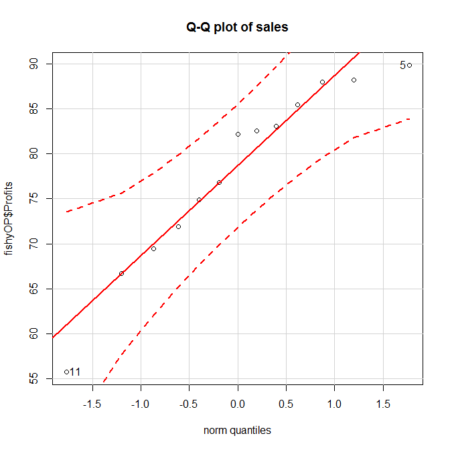
Figure 1. A Q-Q plot, the default command in Rcmdr
Rcmdr: Graphics → Quantile-comparison plot…
After choosing the variable (in this case, Sales), click on Options tab and make additional selections before making the graph. Here, selected normal distribution.
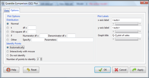
Figure 2. Screenshot of R Commander menu for Q-Q plot
Another version is available in the KMggplot2 package.
Questions
- What is a Q-Q plot used for in statistics?
- Looking at the plot in Figure 1, explain why the confidence lines get further and further away from the straight line.
Quiz Chapter 4.7
Q-Q plots
Chapter 4 contents
3.3 – Measures of dispersion
More about summary statistics.
The statistics of data exploration involve calculating estimates of the middle, central tendency, and the variability, or dispersion, about the middle. Statistics about the middle were presented in the previous section, Chapter 3.1. Statistics about measures of dispersion, and how to calculate them in R, are presented in this page. Use of Z score to standardize or normalize scores is introduced. Statistical bias is also introduced.
Describing the middle of the data gives your reader a sense of what was the typical observation for that variable. Next, your reader will want to know something about the variation about the middle value — what was the smallest value observed? What was the largest value observed? Were data widely scattered or clumped about the middle?
Measures of dispersion or variability are descriptive statistics used to answer these kinds of questions. Variability statistics are very important and we will use them throughout the course. A key descriptive statement of your data, how variable?
Note 1: Data is plural = a bunch of points or values; datum is the singular and rarely used.
Examine the two figures below (Fig 1 and Fig 2): the two sample frequency distributions (put data into several groups, from low to high, and membership is counted for each group) have similar central tendencies (mean), but they have different degrees of variability (standard deviation).
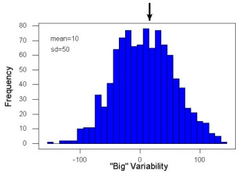
Figure 1. A histogram which displays a sampling of data with a mean of 10 (arrow marks the spot) and standard deviation (sd) of 50 units.
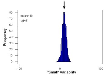
Figure 2. A histogram which displays a sampling of data with the same mean of 10 (arrow marks the spot) displayed in Fig. 1, but with a smaller standard deviation (sd) of 5 units.
Clearly, knowing something about the middle of a data set is only part of the required information we need when we explore a data set; we need measures of dispersion as well. Provided certain assumptions about the frequency of observations hold, estimates of the middle (eg, mean, median) and the dispersion (eg, standard deviation) are adequate to describe the properties of any observed data set.
For measures of dispersion or variability, the most common statistics are: Range, Mean Deviation, Variance, Standard Deviation, and Coefficient of Variation.
The range.
The range is reported as one number, the difference between maximum and minimum values.

Arrange the data from low to high, subtract the minimum, Xmin, from the maximum, Xmax, value and that’s the range.
For example, the minimum height of a collection of fern trees might be 1 meter whereas the maximum height might be 2.2 meters. Therefore, the range is 1.2 meters (= 2.2 – 1).
The range is useful, but may be misleading (as index of true variability in population) if there is one or more exceptional “outlier” (one individual that has an exceptionally large or small value). I often just report Xmin and Xmax. That’s the way R does it, too.
If you recall, we used the following as an example data set.
x = c(4,4,4,4,5,5,6,6,6,7,7,8,8,8,15)The command for range in R is simply range().
range(x)
[1] 4 15
There is apparently no universally accepted symbol for “range,” so we report the statistic as range = 15 – 4 = 11.
You may run into an interquartile range, which is abbreviated as IQR. It is a trimmed range, which means, like the trimmed mean, it will be robust to outlier observations. To calculate this statistic, divide the data into fourths, termed quartiles. For our example variable, x, we can get the quartiles in R
quantile(x)
  0%  25%  50%  75% 100%
 4.0  4.5  6.0  7.5 15.0
Thus, we see that 25% of the observations are 4.5 (or less), the second quartile is the median, and 75% of the observations are less than 7.5. The IQR is the difference between the first quartile, Q1, and the third quartile, Q3.
The command for obtaining the IQR in R is simply IQR(). Yes. You have to capitalize “IQR” — R is case sensitive; that means IqR is not the same as IQR or iqr.
IQR(x)
[1] 3.5
and we report the statistic as IQR = 3.5. Thus, 75% of the observations are within 3.5 points of the median. The IQR is used in box plots (Chapter 4). Quartiles are special cases of the more general quantile; quantiles divide up the range of values into groups with equal probabilities. For quartiles, four groups at 25% intervals. Other common quantiles include deciles (ten equal groups, 10% intervals) and percentiles (100 groups, 1% intervals).
The mean deviation.

Subtract each observation from the sample mean; each  is called a deviate: some observations will be positive (greater than
 ) and some will be negative (less than ).
Take the absolute value of the deviation and then add up the absolute values of the deviations from the mean. At the end, divide by the sample size, n. Large values for this statistic implies that much of the data is spread out, far from the mean. Small values in turn imply that each observation is close to the mean.
Note 2: The mean deviation will always be positive, which is why we take the absolute. By taking the absolute value of each deviate, then the sum is greater than zero. Now, we rarely use this statistic by itself — but that difference is integral to much of the statistical tests we will use. Look for this difference in other equations!
In R, we can get the mean deviation with the mad() function. At the R prompt, then
mad(x)
[1] 2.9652
Population variance and population standard deviation.
The population variance is appropriate for describing variability about the middle for a census. Again, a census implies every member of the population was measured. Equation of the population variance is
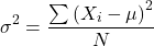
The population standard deviation also describes the variability about the middle, but has the advantage of being in the same units as the quantity (ie, no “squared” term). Equation of the population standard deviation is

Sample variance and sample standard deviation.
The above statements about the population variance and standard deviation hold for the sample statistics. Equation of the sample variance
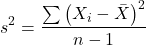
and the equation of the sample standard deviation

Of course, instead of taking the square-root of the sample variance, the sample standard deviation could be calculated directly.
*** QuickLaTeX cannot compile formula:
\begin{align*}s = \sqrt{\frac{\sum \left ( X_{i} - \bar{X} \right )^2}{n-1}\end{align*}

*** Error message:
File ended while scanning use of \align*.
Emergency stop.
n - 1 instead of N. This is Bessel’s correction and we will take a few moments here and in class to show you why this correction makes sense. Bessel’s correction to the sample variance illustrates a basic issue in statistics: when estimating something, we want the estimator (ie, the equation), to be an unbiased value for the population parameter it is intended to estimate.Statistical bias is an important concept in its own right; bias is a problem because it refers to a situation in which an estimator consistently returns a value different from the population parameter for which it is intended to estimate. Thus, the sample mean is said to be an unbiased estimator of the population mean. Here, bias means that the formula will give you a good estimate of the value. This turns out not to be the case for the sample variance if you divide by n instead of n - 1. Now, for very large values of n, this is not much of an issue, but it shows up when n is small. In R you get what you ask for — if you ask for the sample standard deviation, the software will return the correct value; calculators, go to watch out for this — not all of them are good at communicating which standard deviation they are calculating, the population or the sample standard deviation.
Winsorized variances.
Like the trimmed mean and winsorized mean (Ch3.2), we may need to construct a robust estimate of variability less sensitive to extreme outliers. Winsorized refers to procedures to replace extreme values in the sample with a smaller value. As noted in Chapter 3.2, we chose the level ahead of time, eg, 90%. Winsorized values then The winsorized variance is just the sample variance of the winsorized values. winvar() from the WRS2 package.
Making use of the sample standard deviation.
Given an estimate of the mean and an estimate of the standard deviation, one can quickly determine the kinds of observations made and how frequently they are expected to be found in a sample from a population (assuming a particular population distribution). For example, it is common in journal articles for authors to provide a table of summary statistics like the mean and standard deviation to describe characteristics of the study population (aka the reference population), or samples of subjects drawn from the study population (aka the sample population). The CDC provides reports of attributes of for a sample of adults (more than forty thousand) from the USA population (Fryar et al 2018). Table 1 shows a sample of results for height, weight, and waist circumference for men aged 20 – 39 years.
Table 1. Summary statistics mean ( standard deviation) of height, weight, and waist circumference of 20-39 year old men USA.
| Years | Height, inches | Weight, pounds | Waist Circumference, inches |
|---|---|---|---|
| 1999 – 2000 | 69.4 (0.1) | 185.8 (2.0) | 37.1 (0.3) |
| 2007 – 2008 | 69.4 (0.2) | 189.9 (2.1) | 37.6 (0.3) |
| 2015 – 2016 | 69.3 (0.1) | 196.9 (3.1) | 38.7 (0.4) |
We introduced the normal deviate as a way to normalize scores, and which we we will use extensively in our discussion of the normal distribution in Chapter 6.7, as a way to standardize a sample distribution, assuming a normal curve.

For data that are normally distributed, the standard deviation can be used to tell us a lot about the variability of the data:
62.26% of the data will lie between  of
95.46% of the data will lie between  of
99.0% of the data will lie between  of
This is known as the empirical rule, where 68% of the observations will be within one standard deviation, 95% of observations will be within two standard deviations, and 99% of observations will be within three standard deviations.
For example, men aged 20 years in the USA are on average μ = 5 feet 11 inches tall, with a standard deviation of σ = 3 inches. Consider a sample of 1000 men from this population. Assuming a normal distribution, we predict that 623 (62.26%) will be between 5 ft. 8 in. and 6 ft. 2 in. ( ).
Where did the 5 ft. 8 in. and the 6 ft. 2 in. come from /? We add or subtract multiples of standard deviations. Thus, 6 ft. 2 in. = 5 ft. 11 in.  (replace σ = 3) and 5 ft. 8 in. = 5 ft. 11 in.
 (again, replace σ = 3″).
Can generalize to any distribution. Chebyshev’s inequality (or theorem) guarantees that no more than a particular fraction  of observations can be a specified
 standard deviations distance away from the mean ( needs to be greater than 1). Thus, for
 standard deviations, we expect a minimum of 75% of values within (
 ) two standard deviations away from the mean, or for
 , then 89% of values will be within (
 ) three standard deviations from the mean.
Hopefully you are now getting a sense how this knowledge allows you to plan an experiment.
For example, for a sample of 1000 observations of height of men, how many do we expect to be greater than 6 ft. 7 in. tall? Apply the empirical rule and do a little math — 79 inches (6 ft. 7 in) minus 71 inches (the mean) is equal to 8. Divide 8 by 3 (our value of ) you’ll get 2.66667; so, 6 ft. 7 in. tall is about 2.67 X standard deviations greater than the mean. From Chebyshev’s inequality we have  , or 14% of observations less than or greater than the mean (
 ).
Our question asks only about expected number of observations greater than  ; divide 14% in half — we therefore expect about 70 individuals out of 1000 men sampled to be 6 ft. 7 in. or taller. Note we made no assumption about the shape of the distribution. If we assume the sample of observations comes from the normal distribution, then we can apply the Z score: about 4 individuals out of 1000 expected to be from the mean (see R code in Note box). We extend the Z-score work in Chapter 6.7.
Note 4: R code:
round(1000*(pnorm(c(79), mean=71, sd=3,lower.tail=FALSE)),0)
or alternatively
round(1000*(pnorm(c(2.67), mean=0, sd=1,lower.tail=FALSE)),0)
R output
[1] 4
R Commander command
Rcmdr: Distributions → Continuous distributions → Normal distribution → Normal probabilities …, select Upper tail.
Another example, this time with a data set available in R, the diabetic retinopathy data set in the survival package.
data(diabetic, package="survival")
Ages of the 394 subjects ranged from 1 to 58. Mean was 20.8 + 14.81 years. How many out of 100 subjects do we expect greater than 50 years old? With Chebyshev’s inequality we have  , or 25.7% of observations less than or greater than the mean, so about 13. If we assume normality, then Z score (Upper tail) is 28.5% and we expect 28 subjects older than 50. Checking the data set, only eight subjects were older than 50. Our estimate by Chebyshev’s inequality was closer to the truth. Why /? Take a look at the histogram (Ch4) of the ages (Fig 3).
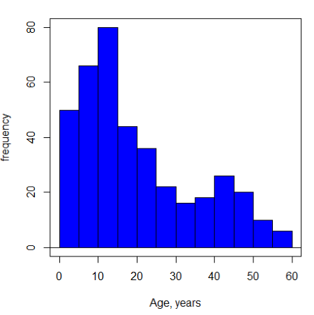
Figure 3. Histogram of ages of subjects in the diabetic retinopathy data set in the survival package.
Doesn’t look like a normal distribution, does it/?.
Z-score or Chebyshev’s inequality, which to use /? Chebyshev’s inequality is more general — it can be used whether the variables is discrete or continuous and without assumption about the distribution. In contrast, the Z score assumes more is known about the variable: random, continuous, drawn from a normally distributed population. Thus, as long as these assumptions hold, the Z score approach will give a better answer. Makes intuitive sense — if we know more, our predictions should be better.
In summary from the above points, and perhaps more formally for our purposes, the standard deviation is a good statistic to describe variability of observations on subjects, it’s integral to the concept of precision of an estimate and is part of any equation for calculating confidence intervals (CI). For any estimated statistic, a good rule of thumb is to always include a confidence interval calculation. We introduced these intervals in our discussion of risk analysis (approximate CI of NNT), and we will return to confidence intervals more formally when we introduce t-tests.
When you hear people talk about “margin of error” in a survey, typically they are referring to the standard deviation — to be more precise, they are referring to a calculation that includes the standard deviation, the standard error and an accounting for confidence in the estimate (see also Chapter 3.5 – Statistics of error).
Corrected Sums of Squares.
Now, take a closer look at the sample variance formula. We see a deviate

The variance is the average of the squared deviations from the mean. Because of the “squared” part, this statistic will always be positive and greater (or typically, equal to) zero. The variance has squared units (eg, if the units were grams, then the variance units are grams2). The sample standard deviation has the same units as the quantity (ie, no “squared” term). The numerator is called a sums of squares, and will be abbreviated as SS. Much like the deviate, will show up frequently as we move forward in statistics (eg, it’s key to understanding ANOVA).
Other standard deviations of means.
Just as we discussed for the arithmetic average, there will be corresponding standard deviations for the other kinds of means. With the geometric mean, one would calculate the standard deviation of the geometric mean, sgm, as
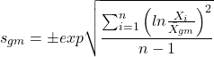
where exp is the exponential function, ln refers to natural logarithm, and  refers to the sample geometric mean.
For the sample harmonic mean, it turns out there isn’t a straight-forward formula, only an approximation (which I will spare you — it involves use of expectations and moments).
Base R, and therefore Rcmdr, doesn’t have built in functions for these, although you could download and install some R packages which do (eg, package NCStats, and the function is geosd() ).
If we run into data types appropriate for the geometric or harmonic means and standard deviations I will point these out; for now, I present these for completeness only.
Coefficient of variation (CV).
An unfortunate property of the standard deviation is that it is related (= “correlated”) to the mean — a fact recognized by Pearson (1896, p 276). Thus, if the mean of a sample of 100 individuals is 5 and variability is about 20%, then the standard deviation is about 1; compare to a sample of 100 individuals with mean = 25 and 20% variability, the standard deviation is about 5. For means ranging from 1 to 100, here’s a plot to show you what I am talking about.
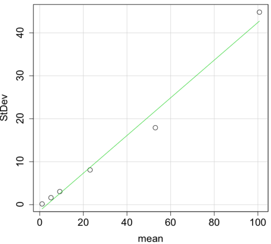
Figure 4. Scatter plot of the standard deviation (StDev) by the mean. Data sets were simulated.
The data presented in the Figure 4 graph were simulated. Is this bias, a correlation between mean and standard deviation, something you’d see in “real” data? Here’s a plot of height in inches at withers for dog breeds (Fig 5). A line is drawn (ordinary linear regression, see Chapter 17) and as you can see, as the mean increases, the variability as indicated by the standard deviation also increases.
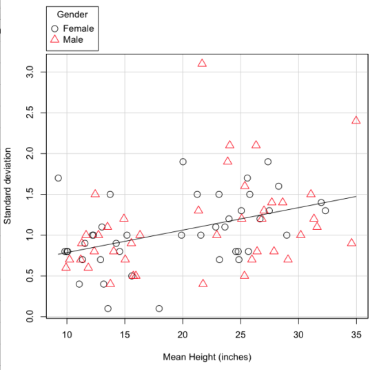
Figure 5. Plot of the standard deviation by the mean for heights of different breeds of dogs.
So, to compare variability estimates among groups when the means also vary, we need a new statistic, the coefficient of variation, abbreviated CV (Pearson 1896). The coefficient of variation is also known as the relative standard deviation, RSD. Many statistics textbooks not aimed at biologists do not provide this estimator (eg, check your statistics book).
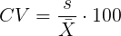
This is simply the standard deviation of the sample divided by the sample mean, then multiplied by 100 to give a percent. The CV is useful when comparing the distributions of different types of data with different means.
Many times, the standard deviation of a distribution will be associated with the mean of the data.
Example. The standard deviation in height of elephants will be larger on the centimeter scale than the standard deviation of the height of mice. However, the amount of variability RELATIVE to the mean may be similar between elephants and mice. The CV might indicate that the relative variability of the two organisms is the same.
The standard deviation will also be influenced by the scale of measurement. If you measure on the mm scale versus the meter scale the magnitude of the SD will change. However, the CV will be the same!
By dividing the standard deviation by the mean you remove the measurement scale dependence of the standard deviation and generally, you also remove the relationship of the standard deviation with the mean. Therefore, CV is useful when comparing the variability of the data from distributions with different means.
One disadvantage is that the CV is only useful for ratio scale data (ie, those with a true zero).
The coefficient of variation is also one of the statistics useful for describing the precision of a measurement. See Chapter 3.4 Estimating parameters.
Standard error of the mean (SEM).
All estimates should be accompanied by a statistic that describes the accuracy of the measure. Combined with the confidence interval (Chapter 3.4), one such statistic is called the standard error of the mean, or SEM for short. For the error associated with calculation of our sample mean, it is defined as the sample standard deviation divided by the square root of n, the sample size.
sem → 
The concept of error for estimates is a crucial concept. All estimates are made with error and for many statistics, a calculation is available to estimate the error (see Chapter 3.4).
Although related to each other, the concepts of sample standard deviation and sample standard error have distinct interpretations in statistics. The standard deviation quantifies the amount of variation of observations from the mean, while the standard error quantifies the difference between the sample mean and the population mean. The standard error will always be smaller than the standard deviation and is best left for reporting accuracy of a measure and statistical inference rather than description.
Questions.
- For a sample data set like
myY <- c(1,1,3,6), you should now be able to calculate, by hand, the
• range
• mean
• median
• mode
• standard deviation
• coefficient of variation - For our example data set,
myX <- c(4,4,4,4,5,6,6,6,7,7,8,8,8,8,8)calculate
• IQR
• sample standard deviation, s
• coefficient of variation - Use the
sample()command in R to draw samples of size 4, 8, and 12 from your example data set stored inmyX. Repeat the calculations from question 4. For examplex4 <- sample(x,4)will randomly select four observations from x, and will store it in the object x4, like so (your numbers probably will differ!)x4 <- sample(x,4); x4 [1] 8 6 8 6 - Repeat the exercise in question 4 again using different samples of 4, 8, and 12. For example, when I repeat sample(
x,4) a second time I getsample(x,4) [1] 8 4 8 6 - For Table 1, determine how many multiples of the standard deviation for observations greater than 95-percentile (eg, determine the observation value for a person who is in the 95-percentile for Height in the different decades, etc.
- Calculate the sample range, IQR, sample standard deviation, and coefficient of variation for the following data sets
• Height in inches of mothers,mom <- c(67, 66.5, 64, 58.5, 68, 66.5) #(data from GaltonFamilies in R package HistData)
and fathers,dad <- c(78.5, 75.5, 75, 75, 74, 74) #(data from GaltonFamilies in R package HistData)
• Carbon dioxide (CO2) readings from Mauna Loa for the month of December for
years <-c (1960, 1965, 1970, 1975, 1980, 1985, 1990, 1995, 2000, 2005, 2010, 2015, 2020)years <-c (1960, 1965, 1970, 1975, 1980, 1985, 1990, 1995, 2000, 2005, 2010, 2015, 2020) #obviously, do not calculate statistics on years; you can use to make a plotco2 <- c(316.19, 319.42, 325.13, 330.62, 338.29, 346.12, 354.41, 360.82, 396.83, 380.31, 389.99, 402.06, 414.26) #(data from Dr. Pieter Tans, NOAA/GML (gml.noaa.gov/ccgg/trends/) and Dr. Ralph Keeling, Scripps Institution of Oceanography (scrippsco2.ucsd.edu/))
• Body mass of Rhinella marina (formerly Bufo marinus) (see Fig. 1),bufo <- c(71.3, 71.4, 74.1, 85.4, 85.4, 86.6, 97.4, 99.6, 107, 115.7, 135.7, 156.2)
Quiz – Chapter 3.3
Measures of dispersion
Chapter 3 contents