16 – Correlation, Similarity, and Distance
Introduction
We continue with our discussion and introduction of inferential statistics. Recall that as we analyze a data set, we generally want to begin by describing it (central tendency, measures of variability), and we also want to plot the data. To begin our introduction to correlation and regression, first we describe how to produce graphs to help show linear association or in some cases, cause and effect — the latter perhaps the primary reason for using regression.
Graphical representation
The previous statistical procedures we have examined have used one or more categorical or qualitative variables (Chapter 3). For example,
- Chi-Square Analyses: variables are all categorical, including the response variable (Chapter 9).
- T-tests: one categorical (Factor) variable and one (Dependent, Outcome, Response) variable that was continuous or interval scale (Chapter 8.5, 10).
- ANOVA Analyses: one or more variables are categorical (Factors, the independent variables) and one (Dependent, Outcome, Response) variable that was continuous or interval scale (Chapter 12, 14).
The convention in graphing ANOVA (or Chi-Square) is to use the Factor or Independent variables as the
X-axis and to have the dependent variable (Response) as the Y-axis. We called these bar charts (Chapter 4.1).
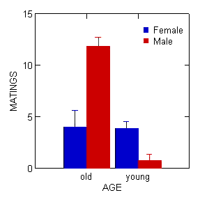
Figure 1. Bar chart with error bars.
Box plots (Chapter 4.3) are also useful, and perhaps the preferred choice to display this type of comparison (one involving groups) (Fig 2).
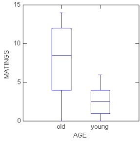
Figure 2. Box plots.
In correlation (and regression) analyses we will have two or more continuous or interval scale variables. To show relationships among continuous variables, a scatter plot, also called an X-Y plot, works well (Chapter 4.5).
In correlation, no causation is implied, so either variable can be placed on the X-axis. The convention of graphing in regression is to place the independent variable as the X-axis and the dependent variable as the Y-axis (Fig 3). Another consideration: if one variable is considered fixed and the other random, then the fixed variable would be assigned to the horizontal axis.
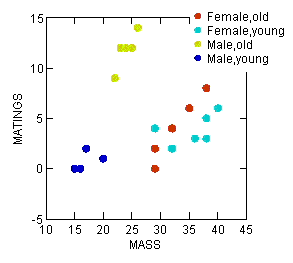
Figure 3. Scatterplot with groups
To produce a scatterplot (also called an X-Y plot) in Rcmdr, select Graph → Plot → and select the Y and X variables. Use a combination of Options, Frame, and Edit Attributes selections to modify the default graph.
Suggested homework
Homework 10: Correlation.
Quizzes in this chapter
A total of 64 questions among the several subchapters, a mix of true or false and multiple choice question format.
Chapter 16 contents
9 – Inferences, Categorical Data
Introduction
We introduced the chi-square distribution in 6.9 – Chi-square distribution. No doubt you have already been introduced to chi-square ( ) tests (click here correct pronunciation), particularly if you’ve had a genetics class, but perhaps you were not told why you were using the test, as opposed to some other test, for example t-test, ANOVA, or linear regression.
Chi-square analyses are used in situations of discrete (ie, categorical or qualitative) data types. When you can count the number of “yes” or “no” outcomes from an experiment, then you are talking about a problem. In contrast, continuous (ie, quantitative) data types for outcome variables would require you to use the t-test (for two groups) or the ANOVA-like procedures (for two or more groups). Chi-square tests can be applied when you have two or more treatment groups.
Two kinds of chi-square analyses
(1) We ask about the “fit” of our data against predictions from theory. This is the typical chi-square that student’s have been exposed to in biology lab. If outcomes of an experiment can be measured against predictions from some theory, then this is a goodness of fit (gof) . Goodness of fit is introduced in Ch09.1.
Note 1: The fit concept in statistics is simply how well a statistical model explains the data. As we go forward, this concept will appear frequently.
(2) We ask whether the outcomes of an experiment are associated with a treatment. These are called contingency table problems, and they will be the subject of the next lecture. The important distinction here is that there exists no outside source of information (“theory”) available to make predictions about what we would expect. Contingency tables are introduced in Ch09.2.
Suggested homework
Quizzes in this chapter
A total of 45 questions among the several subchapters, a mix of true or false and multiple choice question format.
Chapter 9 contents
- Introduction
- Chi-square test: Goodness of fit
- Chi-square contingency tables
- Yates continuity correction
- Heterogeneity chi-square tests
- Fisher exact test
- McNemar’s test
- References and suggested readings