7.2 – Epidemiology basics
Introduction
A principle aim of epidemiology is to identify frequency and causes of illnesses. Kinds of evidence gathered range from case studies to randomized controlled trials, to meta-analysis and systematic reviews. In turn, how these kinds of evidence are evaluated and turned into policy recommendations generally accounts for additional concerns eg, GRADE – Grading of Recommendations Development, Assessment and Evaluation Schünemann et al 2023). Learning about conditional probability in biostatistics is essential for discussing evidence because it provides a rigorous framework for updating strength of evidence based on new, specific information. It allows for the objective assessment of how new evidence — results from a clinical test — influences the likelihood of a hypothesis — presence/absence of disease for a patient. Conditional probability analysis allows interpretation of a positive test result in the context of disease prevalence, which may lead to the paradoxical conclusion that a test with high sensitivity applied to a person belonging to a low at risk group is more likely a false positive than evidence of a true positive.
Thus, to introduce conditional probability, I have elected to push you into epidemiology and risk analysis. We introduced epidemiology definitions and here, we build on basic terminology of epidemiology. Epidemiology is the study of the causes and distribution of health-related events in a population. It is has been called the basic science of public health (p. 16, Decker 2008).
Prevalence rate
Prevalence of a disease (condition), is defined as the proportion of the population that has the disease (condition) at a point or duration in time. The prevalence statistic is the ratio of the number of existing cases divided by the total population.
For example, prevalence of Type 2 diabetes in Hawai`i. The 2020 populations was about 1.4 million. A survey was conducted on a random of 1000 individuals and 80 were reported to have Type 2 diabetes. What is the estimated prevalence of Type 2 diabetes in Hawai`i?
Start from perspective — what if we actually have something close to a census count? For the actual estimates, see the report at the Hawaii State DOH website. With every estimate of a statistic, we need a confidence interval (CI). An approximate (good for large samples) formula for the 95% CI of prevalence is

where  is the 2010 prevalence in the population (8.3%), N is the population size (1,360,301), and z is the standard normal probability. For a 95% CI, then we want z95%.
If you recall, we can get this from our standard normal probability table, or directly from R. We want to know z that is in the ± 2.5% tails of the distribution (that’s 0.05 ÷ 2, see Ch 8.4 – Tails of a test). Our R code then is
qnorm(c(0.025), mean=0, sd=1, lower.tail=FALSE)
which returns
[1] 1.959964
You should confirm that setting lower-tail = TRUE yields -1.96 (rounded).
Alternately, if using Rcmdr: Distributions → Continuous distributions → Normal distribution → Normal quantiles… (Fig 1).
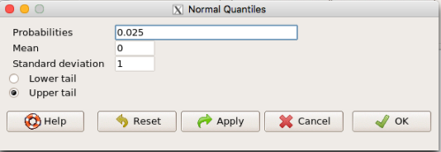
Figure 1. R Commander popup menu for Normal quantiles.
Thus, for our example, the 95% CI was ( ; our confidence in our estimate of the prevalence of diabetes in Hawaii is between 8.25% and 8.35%. Again, note that for our purposes it is OK to calculate the approximate confidence interval, replace
 with
 (for large N, the differences are observed in the 0.001 decimal).
Prevalence: R code
Rather than census counts, more likely we have results of smaller surveys. We use the epi.conf() function from the epiR package. Code adapted from example provided in epiR_descriptive vignette.
Note 1: Many R packages include vignettes, which, together with the package manual, is often helpful to understand what a function is intended to do and how to get the most from the function. R code to call all vignettes available for a package, eg, epiR:
vignette(package="epiR")
which will return names of available vignettes. For epiR, these are
epiR_descriptive Descriptive epidemiology (source, html)
epiR_surveillance Disease surveillance (source, html)
epiR_measures_of_association Measures of association (source, html)
epiR_sample_size Sample size calculations (source, html)
To call up the vignette we need for this example,
vignette("epiR_descriptive", package="epiR")
which brings up the page (assuming you installed the html help files during installation of base R).
library(epiR)
pop.Hawaii = 1.4e06
pop.Survey = 1000
type2.Survey = 80
Table.2 <- as.matrix(cbind(type2.Survey, pop.Survey))
epi.conf(Table.2, ctype = "prevalence", method = "exact", N = pop.Hawaii, design = 1, conf.level = 0.95) * 100
R output
   est    lower    upper
1    8 6.394198 9.857978
Thus, estimated Type 2 diabetes prevalence from the survey was 8, with 95% confidence interval 6.4 to 9.9 cases per 100 individuals. From 2020 U.S. Census, Hawai`i population was 1,455,271.
Note 2: Type 2 diabetes is one of many conditions for which prevalence is greater among Native Hawaiian and Pacific Islander populations compared to other groups in Hawai’i (Galinski et al 2016); these are called health disparitiess.
Incidence rate
Incidence of a disease (or condition) is defined as the occurrence of new cases of a disease. The simplest way to view incidence is that if everyone was followed for the same period of time, then incidence rate is the number of new cases since the start of the study divided by the total population. This is too simplistic, so we define a better metric called person-time. Incidence rate (IR) is then the ratio of the number of new cases divided by total person-time.
Again, incidence rate is an estimate. Therefore, we need a confidence interval. Assuming the population is large, then confidence interval can be calculated as

where IR is the incidence rate, T is the person-time, N is the number of events or cases, and z again is the standard normal probability (z ± 1.96 for 95% confidence interval).
For our example, N = 3 cases, T = 236 p-d, so 95% CI is (11.3%, 14.1%).
Person-time
Person-time can be days, months, years. Person-time is best defined with an example.
Five men join a study that will last 70 days. These men were selected because they had suffered a myocardial infarction (MI) and at the start of the study, they receive the same treatment. The outcome of the study is whether or not the subjects suffer a second MI.
The results are shown below
Subject A, 53 days
Subject B, 70 days
Subject C, 24 days
Subject D, 70 days
Subject E, 19 days
Add up the person days,

Now calculate the incidence rate,

that’s 3 cases (A, C, E) divided by 236 p-d = 0.0127. Multiply this by 1000 and we get our final answer for the incidence rate, 12.7 per person-days.
Incidence rate: R code
Incidence rate of myocardial infarction (MI) study. Code adapted from example provided in epiR_descriptive vignette.
ncas = 3
ntar = 236
tmp <- as.matrix(cbind(ncas, ntar))
epi.conf(tmp, ctype = "inc.rate", method = "exact", N = 1000, design = 1, conf.level = 0.95) * 1000
R output
          est    lower    upper
ncas 12.71186 2.621492 37.14946
The incidence rate of myocardial infarction was 12.7 (95% CI 2.6 to 37.2) cases per 1000 person-days.
Age-specific rates
Incidence or prevalence rates may be reported for specific age groups. For example, we can distinguish between number of live births in Hawaii in 2017, and numbers of live births by age group of the mother.
Age-adjusted rates
If populations with different age demographics, then the convention is to adjust the populations to a standard reference population with known age and other demographic properties. For example, the CDC uses the 2000 census as the standard population (CDC definitions, age adjustment, retrieved January 2023).
Questions
- Calculate the confidence interval of type 2 prevalence in Hawai`i with the 2020 census population value. How much did it change?
- Recalculate the confidence interval for a 99% confidence interval. Which estimate communicates greater confidence in the estimate?
Quiz
Quiz Chapter 7.2
Epidemiology basics
Chapter 7 contents
6.4 – Types of probability
Introduction
By probability, we mean a number that quantifies the uncertainty associated with a particular event or outcome. If an outcome is certain to occur, the probability is equal to 1; if an outcome cannot happen, the probability is equal to zero. Most events we talk about in biology have probability somewhere in between.
A basic understanding, or at least an appreciation for probability is important to your education in biostatistics. Simply put, there is no certainty in biology beyond simple expectations like Benjamin Franklin’s famous quip about “death and taxes…”
Discrete probability
You are probably already familiar with discrete probability. For example, what is the probability that a single toss of a fair coin will result in a “heads?” The outcomes of the coin toss are discrete, categorical, either “heads” or “tails.”
Note 1: Obviously, this statement assumes a few things — coin tossed not in a vacuum, for example. We assume a fair coin — equal chance heads or tails. Fair coins have two sides; tossing a coin we expect “heads” or “tails,” but rarely, some coin types may land and come to rest on edge or side (eg, USA nickels). We still consider the coin toss having binary outcomes, by definition, even though a coin may land on edge about one toss in six thousand (Murray and Teare 1993) because the exception is extremely rare. h/t Dr. Jerry Coyne.
And for ten tosses of the coin? And more cogently, what is the probability that you will toss a coin ten times and get all ten “heads?” While different in tone, these are discrete outcomes. An important concept is independence. Are the multiple events independent? In other words, does the toss of coin on the first attempt affect the toss of the coin on the second attempt and so on up to the tenth toss? At least in principle the repeated tosses are independent so to find the probability you just multiply each event’s probability to get the total.
In contrast, if one or more events are not independent but somehow influence the behavior of the next event, then you add the probabilities for each dependent event. We can do better than simply multiply or add events one at a time; depending on the number of discrete outcomes it is very likely that someone has already calculated all possible outcomes and come up with an equation. In the case of the tossing of two coins this is a binomial equation problem and repeat tosses can be modeled by use of the Bernoulli distribution.
Now, try this on for size. What is the probability that the next child born at Kapiolani Medical Center in Honolulu will be assigned female?
We just described a discrete random variable, which can only take on discrete or “countable” numbers. This distribution of values is the probability mass function. The probability of a one fatal airline accident in a year exactly on 20.1 is practically zero (the area under a point along the curve is zero), so we can get the probability of a range of values around the point as our answer.
Continuous probability
Many events in biology are of degree, not kind. It is kind of awkward to think about it, but for a sample of adult house mice drawn from a population, what is the probability of obtaining a mouse that is 20.0000 grams (g) in weight? Each possible value of body mass for a mouse is considered an event, just like in our example of tossing a coin. But clearly, we don’t expect to get a lot of mice that are exactly 20.0000 g in weight. For variables like body mass, the type of data we collect is continuous, and the probability values need to be rethought along a continuum of possible values and, in turn, how likely each value is for a mouse. Although it is theoretically possible that a mouse could weigh ten pounds, we know by experience that this is impossible. Adult mice weigh between 15 and 50 g or there about.
We just described a continuous random variable, which can take on any value between a specific interval of values. This distribution of values is the probability density function (PDF). The probability of a mouse’s weight falling exactly on 20.1 is practically zero (the area under a point along the curve is zero), so we can get the probability of a range of values around the point as our answer.
In statistical inference, following our measurements of the variables from our sample drawn from a population, we make conclusions with the following kind of caveat: “the mean body mass for this strain of mouse is 20 g.” That is our best estimate of the mean (middle) for the population of mice, more specifically, for the body mass of the mice. Here, the variable body mass is more formally termed a random variable. This implies that there is in fact a true population mean body mass for the mice and that any deviations from that mean are due to chance.
In statistics we don’t settle for a single point estimate of the population mean. You will find most reporting of estimates of random variables is accompanies by a statement like, the mean was 20g with a 95% probability that the true population mean is between 18.9 and 21 g. This is called the 95% confidence interval for the mean and it takes into account how good of an estimate our sample is likely to be relative to the true population value. Not only are we saying that we think the population mean is 20g, but we’re willing to say that we are 95% certain that the true value must be between a lower limit (18.9 g) and and upper limit (21 g). In order to make this kind of statement we have to assume a distribution that will describe the probability of mouse weights. For many reasons we usually assume a normal distribution. Once we make this assumption we can calculate how probable a particular weight is for a mouse.
We introduced how to calculate Confidence Intervals in Chapter 3.4 and will extend this in any chapter that introduces an estimation.
Types of probability
To begin refining our concept of probability, it is sometimes useful to distinguish among kinds of probabilities:
- between theoretical and empirical;
- between subjective and objective.
In most cases, including your statistics book, we would begin our discussion of probability by talking of some probabilities for events we’re familiar with.
- The theoretical probability of heads appearing the next time you flip a fair coin is 1/2 or 50%. As long as we’re talking about a fair coin, the probability of a heads appearing each time you flip the coin remains 50%. We can check this by conducting and experiment: out of 10 tosses, how many heads appear? The answer would be an empirical probability, and we understand the chance in an objective manner (no interpretation needed).
- The theoretical probability that a “5” will appear on the face of a fair dice after a toss is 1/6 or 16.667%. Again, as long as we’re talking about a fair dice, the probability of a “5” appearing each time you roll the dice remains 16.667%.
- The probability that at birth, a human baby’s sex will be male about 1/2 or 50%. This is an empirical probability based on millions of observations. Changes in technology, and ethical standards notwithstanding, the probability will remain the same.
- The probability of the birth of a Downs syndrome baby is 1/800, but increases with age until by age 45, the chance is 1/12. Again, these are empirical and objective.
- The probability of winning the Publisher’s Clearing House Sweepstakes is about 1 in 100 million. This probability is theoretical, it is also objective; however, by adding lots of twists to the game, by having multiple opportunities and by giving the appearance that a person must purchase a magazine, some players perceive their chances as increasing or decreasing by their efforts (=subjective).
R and distributions
R offers access to many named distributions. R generally provides four functions available for each.
density (d):the probability density function (PDF) for continuous distributions or the probability mass function (PMF) for discrete distributions.
probability (p): the cumulative distribution function (CDF), which is the chance (probability) of a random variable being less than or equal to a given value
quantile (q): the quantile function (inverse CDF), which returns the value at a given probability
r: draw random numbers from the specified distribution.
Examples of functions for the normal distribution then, are: dnorm(), pnorm(), qnorm(), and rnorm().
Coding example: Find the PDF for x = 0 in a standard normal distribution. # Find the PDF value for x = 0 in a standard normal distribution (mean=0, sd=1)
dnorm(x = 0, mean = 0, sd = 1)
R output
0.398942280401433
Thus, we conclude the chance that x = 0 is about 40%.
Note 2: Technically it’s not the chance that x is exactly 0 — it refers to the chance that the random variable falls within fractionally small interval around that value. That’s the calculus foundation for probability speaking.
Coding example: Find the probability that for x is equal to -1.2 or less in a standard normal distribution.
pnorm(q = -1.2, mean = 0, sd = 1, lower.tail = TRUE)
R output
0.115069670221708
Thus, we conclude the chance that x is equal to or less than -1.2 is about 11.5%.
Coding example: Assuming normal distribution of test scores, what score will 50% of students score? Find the probability that for x is equal to -1.2 or less in a standard normal distribution.
qnorm(0.5, mean = 75, sd = 10)
R output
75
As expected, at 50% it returns the mean. Now, confirm that the lower 25% and upper 75% are 68.26 and 81.75, respectively.
Last coding example, draw random sample of three scores from the same exam.
rnorm(3, mean = 75, sd = 10)
R output
-
66.0384856946112
-
69.1887923903669
-
77.6342297053815
R Commander: Distributions menus give four options
- Quantiles
- Probabilities
- Plot
- Sampling
Note 3: Looking for more examples? These kinds of problems are common skill-based questions one finds in any statistics course. Homework 3: Distributions & Probability in Mike’s Workbook for Biostatistics offers several additional examples to work through. Additional examples are provided in Chapter 6.5 and Chapter 6.6.
Questions
1. Define and distinguish, with examples
- discrete and continuous probability
- theoretical and empirical probability
- subjective and objective probability
Quiz Chapter 6.4
Types of probability
Chapter 6 contents
- Introduction
- Some preliminaries
- Ratios and proportions
- Combinations and permutations
- Types of probability
- Discrete probability distributions
- Continuous distributions
- Normal distribution and the normal deviate
- Moments
- Chi-square distribution
- t distribution
- F distribution
- References and suggested readings