6.2 – Ratios and probabilities
Introduction
One common objective of a research project is comparison between quantities: one effective way to communicate a comparison is to construct a ratio. Ratios provide a standardized way to compare different data sets. The purpose of this page is introduce the wealth of types of ratios used for quantification of comparisons, from indexes to ratios.
Let’s review our definitions again. An event is some occurrence. As you know, a ratio is one number, the numerator, divided by another called the denominator. A proportion is a ratio where the numerator is a part of the whole. A rate is a ratio of the frequency of an event during a certain period of time. A rate may or may not be a proportion, and a ratio need not be a proportion, but proportions and rates are all kinds of ratios. If we combine ratios, proportions, and/or rates, we construct an index.
Ratios
Yes, data analysis can be complicated, but we start with this basic idea. Much of the statistics is based on frequency measures, eg, ratios, rates, proportions, indexes, and scales.
Ratios are the association between two numbers, one random variable divided by another. Ratios are used as descriptors and the numerator and denominator do not need to be of the same kind. Business and economics are full of ratios. For example, return on investment (ROI), eg, earnings equals net income divided by number of shares outstanding, the Price-Earnings, or P/E ratio, is the ratio of the price of a stock to the earnings per stock, as well as many others are used to summarize performance of a business, and to compare performance of one business against another.
Note 1: ROI also stands for region of interest — a sample in a data set identified by the analyst for a particular interest. Often refers to a specific area in an image.
Ratios are deceptively convenient way to standardize a variable for comparisons, ie, how many times one number contains another. For example, when estimating bird counts for different areas, or different birding effort (intensity, time searched), we may correct counts by accounting for area in which counts were made or the total time spent counting, for a per-unit ratio (Liermann et al 2004).
Practice: There were 1,326 day undergraduate students enrolled in 2014 at Chaminade University of Honolulu and the Sullivan Library added 8469 new items (ebooks, journals, etc,) to its collection during 2014. What is the ratio of new items per student?

Data collected from Chaminade University website at www.chaminade.edu on 3 July 2014.
Practice: For another example, what is ratio of annual institutional aid a student at Chaminade University may expect to receive compared to a student at Hawaii Pacific University?

Thus, in 2014, Chaminade offered more than twice the institutional aid to its students then does HPU (both institutions are private universities, data from retrieved on 3 July 2014 from www.cappex.com).
Relative change, Fold-change and orders of magnitude
It’s common practice to report on the amount of change between two quantities recorded over time. Relative change (often percentage) describes change relative to an initial value. Relative change in root length b
To make percent increase (decrease), simply multiple 100%.
(1) 
The ratio between two quantities, eg, to compare mRNA expression levels of genes from organisms exposed to different conditions, researchers may report fold-change. Fold change is often reported as log base 2 change.

Why log base 2? Symmetry and ease of reporting. A doubling becomes +1 and a halving becomes -1. Without log transformation, doubling is +2, but having is +0.5.
Relative change is useful for reporting percent changes, fold change for ratios, although if the change is small in amount, then relative change can be misleading, eg, value goes from five to ten, then the relative change is 100%, but effectively, a very small change in absolute units. Similarly, fold change becomes a large, but likely meaningless comparison, if the denominator is close to zero.
An example of calculation of fold change. Rates of the expression from cells exposed to heavy metal divided by expression under basal conditions. Gene expression under different treatments may be evaluated by calculating fold-change as the log base2 of the ratio of expression of a gene for one treatment divided by expression of same gene from control conditions. Copper is an essential trace element, but excess exposure to copper is known to damage human health, including chronic obstructive pulmonary disease. One proposed mechanism is that cell injury promotes an epithelial-to-mesenchymal shift. In a pilot study (N.I.H. INBRE P20RR016467), we investigated gene expression changes by quantitative real-time polymerase chain reaction (qPCR) in a rat lung Type II alveolar cell line exposed to copper sulfate compared to unexposed cells. Record cycle threshold values, CT, for each gene, where CT is number of cycles required for the fluorescent signal to exceed background levels; CT is inversely proportional to amount of cDNA (mRNA) in the sample. Genes investigated were ECAD, FOXC2, NCAD, SMAD, SNAI1, TWIST, and VIM, with ATCB as reference gene. ECAD expression is marker of epithelial cells, whereas FOXC2, NCAD, SNAI1, TWIST, and VIM expression marker of mesenchymal cells. After calculating  values, geometric means of normalized values of three replicates each are shown in Table 1.
Note 2: The  is a relative change quantification that relates the PCR signal of the normalized gene of interest (GOI) transcript in a treatment group to another sample, eg, an untreated control. is now a widely applied method to analyze the relative changes in gene expression from real-time quantitative PCR experiments (relevant papers on the analysis method, Livak and Schmittgen (2001) and Schmittgen and Livak (2008) have been cited more than 230K times, Pubmed 2026. See also Rao et al (2013).)
Log-transform, introduced in Ch03.2, was used because gene expression levels vary widely on the original scale and any log-transform will reduce the variability. log-base 2 specifically was used for fold-change in particular because it is easy to interpret (eg, see discussion in Bergemann and Wilson 2011 and Corliss et al 2024), and provides symmetry (all log-transforms provide this symmetry). For example, log(1/2, 2) returns -1, while log(2/1, 2) returns +1. Thus, base 2, we see a decrease by half or doubling of original scale is a fold change of  . In contrast,
log(1/2, 10) returns -0.301, while log(2/1, 10) returns +0.301 — which is perfectly accurate, but deceptive to interpret.
log-base 2 is commonly employed to calculate the number of bits — binary digits — for a given number of values. For example, 8 bits (0 – 7), then log2(8-1), and R returns 2.807355. Round, add 1, and the number of bits is3. Related R code, if want to calculate and print te binary representation of of a number, eg, 8, try
myBits <- intToBits(8)
paste(as.character(myBits),collapse="")
On a more casual note, log-base 2 is useful to calculate number of rounds for a single-elimination playoff tournament, eg, NCAA men’s and women’s basketball tournament or March Madness (NCAA). As of 2025, 60 teams are invited, plus the four winning teams from four play-in games, for a total of 64 teams. The number of rounds is log2(64) and R returns 6. These six are referred to as First Round, Second Round, Sweet Sixteen, Elite Eight, Final Four, and the Championship Game. The play-in games are referred to as the”First Four.” The function draw_bracket() of R package SwimmeR can be used to plot a simple playoff bracket.
Table 1. Mean and fold change of gene expression values from qPCR for several genes from a rat lung cell line.*
| Control | Copper-sulfate | Fold change | |
| ECAD | 34.6 | 35.7 | 0.6 |
| NCAD | 28.5 | 24.0 | 27.2 |
| SMAD | 29.5 | 25.0 | 28.2 |
| SNAI1 | 25.5 | 28.1 | 0.2 |
| FOXC2 | 27.6 | 27.0 | 1.9 |
| VIM | 23.1 | 16.4 | 134.4 |
| TWIST | 25.1 | 22.9 | 5.6 |
* INBRE funding, P20RR016467.
At face value, following four hour exposure to copper sulfate in media, some evidence that the epithelial cell line adopted gene expression profile of mesenchyme-like cells. However, weakness of fold-change is clear from Table 1: the quantity is sensitive to small values. ECAD expression in the cell line is low, thus high numbers of PCR cycles (mean = 36) and treated cells not much fewer (mean = 34.4).
Note 3: Calculation of is included. Geomean CT were
| Control | CuSO4 | |
| ACTB | 32.2 | 32.5 |
| NCAD | 28.5 | 24.0 |
For control cells, 
For treatment cells, 
and 
log2, 
table value differs by rounding
Orders of magnitude
In addition to fold change, order of magnitude is another common way to compare quantities. While fold change returns the multiplier between two numbers, order of magnitude generally refers to differences in multiples of ten, logarithmic.

Thus, a difference of one order of magnitude is the number multiplied by 101, three orders of magnitude is the number multiplied by 103, and so on. A change from 10 to 100 is a one order of magnitude increase; the same change, 10 to 100, is a ten-fold change. It’s a difference of scale. If a person’s salary increases by 3%, from $49K to $50,470, reporting this as an “order of magnitude” increase is nonsensical as a communication device (magnitude of change is just 0.01). By contrast, fold change for the same increase would be 1.03 — also indicative of a negligible increase, but a cleaner representation.
Rates
Rates are a class of ratios in which the denominator is some measure of time. For example, the four year graduation rate of some Hawaii universities are shown in Table 2.
Table 2. Percent students graduation with bachelor’s degrees within four years or six years (cohort 2014, data source NCES.ed.gov)
| School | Private/Public | Four-year, Percent graduation |
Six-year, Percent graduation |
| Chaminade University | Private (non-profit) | 43 | 58 |
| Hawaii Pacific University | Private (non-profit) | 31 | 46 |
| University of Hawaii – Hilo | Public | 15 | 38 |
| University of Hawaii – Manoa | Public | 35 | 62 |
| University of Hawaii – West Oahu | Public | 16 | 39 |
| University of Phoenix | Private (for profit) | 0 | 19 |
Examples of rates
Rates are common in biology. To name just a few
- Basal metabolic rate (BMR), often measured by indirect calorimetry, reported in units kiloJoules per hour.
- Birth rates and mortality (death) rates, components of population growth rate.
- Extinction rate, how often over a given time species go extinct.
- Growth rate, which may refer to growth of the individual (somatic growth rate), or increase of number of individuals in a population per unit time.
- Molecular clock hypothesis, rate of amino acid (protein) or nucleotide (DNA) substitution is approximately constant per year over evolutionary time.
- Mutation rate, frequency of new mutations in a DNA sequence of an organism over time.
- Photosynthetic rate, convert light energy into chemical energy.
- Phred quality score, error rates of incorrectly called nucleotide bases by the sequencer.
Proportions
Proportions are also ratios, but they are used to describe one part to the whole. For example, 902 women (self-reported) day undergraduate students enrolled in 2014 at Chaminade University in Honolulu, Hawaii.
Practice: Given that the total enrollment for Chaminade in 2014 was of 1,326, calculate the proportion of female students to the total student body.

More practice: A common statistic in agriculture is germination percentage, count the number of seeds that sprout over a period of time divided by total number of seeds planted multiplied by 100. Figure 1 shows an example of a germination trial for five tomato seeds. Seed in position 3 (left to right 1 – 5) failed to germinate, whereas the other four seeds display range of seedling growth. (A seed coat is observed next to plant 2.)

Figure 1. Example planting of five tomato seeds, day 5, on agar Petri dish (M. Dohm).
Observations conducted over 10 days. Germination defined as evidence of radicle by day 10. Data collected by student for biostatistics project. A random sample of results from three plates is presented in Table 3.
Table 3. Germination of tomato seeds on agar Petri dishes.
| Plate* | 1 | 2 | 3 | 4 | 5 |
| 18 | Yes | No | Yes | Yes | Yes |
| 13 | Yes | Yes | Yes | No | Yes |
| 20 | No | Yes | Yes | Yes | Yes |
* Random sample of three plates drawn from among 30 plates.
We calculate the percent germination for the 15 seeds planted as

Thus, for the sample of plates the germination percent was 80%, which, coincidently, is the same result if germination percent was calculated for the five seeds displayed in Figure 1.
Beginning in Chapter 7 – Probability, Risk Analysis, we introduce and use a number of proportions, for example incidence and prevalence are proportions, as is PPV — positive predictive value. Sensitivity and specificity are both proportions and also qualified as indexes.
Comparing proportions
In some cases you may wish to compare two proportions or two ratios. The hypothesis tested is the difference between the two ratios, and the test is if the confidence interval of the difference includes zero. If it does, then we would conclude there is no statistical difference between the two proportions. In R, use the prop.test function. For example, 63 women were on team sport rosters at Chaminade in 2014, a proportion of 59% of all student athletes (n = 106). Recall from the example above that women were 68% of all students at Chaminade University. Title IX compliance requires that a university “maintain policies, practices and programs that do not discriminate against anyone on the basis of gender” (NCAA, INCLUSION AND BELONGING Championing Women in Sports). In terms of athletic programs, then, universities are required to provide participation opportunities for women and men that are substantially proportionate to their respective rates of enrollment of full-time undergraduate students.
Consider Chaminade University: Is there a statistical difference between proportion of women athletes and their proportion of total enrollment? We introduce statistical inference in Chapter 8, but for now, this is a test of the null hypothesis that the difference between the two proportions is zero.
At the R prompt type (remember, anything after the # sign is a comment and ignored by R).
women = c(62,902)  #where 62 is the number of women athletes and 902 is the number of women students
students = c(106,1326)  #106 is the number of student athletes and 1326 is all students
prop.test(women,students)  #the default is a two-tailed test, ie, no group differences
And R returns
2-sample test for equality of proportions with continuity correction
 data: women out of students
X-squared = 3.6331, df = 1, p-value = 0.05664
alternative hypothesis: two.sided
95 percent confidence interval:
 -0.197532407 0.006861073
sample estimates:
 prop 1 prop 2
0.5849057 0.6802413
What is the conclusion of the test?
When you compare two groups, you’re asking whether the two groups are equal (the null hypothesis). Mathematically, that’s the same as saying the difference between the two groups is equal to zero.
First check the lower and upper limits of the confidence interval. A confidence interval is one way to report a range of plausible values for an estimate (see Ch 7.6 – Confidence intervals). It’s called a confidence interval because a probability is assigned to the range of values; a 95% confidence interval is interpreted as we’re 95% certain the true population value is somewhere between the reported limits. For our Chaminade University Title IX question, recall that we are asking whether the value of zero is included. The lower limit was -0.1975 and some change; the upper limit was 0.0068 and some change. Thus, zero is included and we would conclude that there was no statistical difference between the two proportions.
The second relevant output to look at is the p-value, or probability value. If the p-value is less than 5%, we typically reject the tested hypothesis. We will talk more about p-values and their relationship to inference testing in Chapter 8; for now, pay attention to the confidence interval (introduced in Chapter 3.4); if zero is included, then we conclude no substantial differences between the two proportions.
Indexes
Indexes are composite statistics that combine indicators. They condense complex diagnostic performance data into a single, universally understood numerical indicator.
Indexes are common in biology, and well-known business and economics indexes are reported on every day, eg, Dow Jones Industrial average combines stock prices from 30 companies listed on the New York Stock Exchange and the CPI, or Consumer Protection Index, constructed by the US Bureau of Labor Statistics from a “market basket of consumer goods and services, used by the government and other institutions to track inflation. The CPI itself is made up of numerous indexes to account for regional price differences and other factors.
Some indexes presented in this book include
- Grade point average
- Body Mass Index (BMI)
- Comet assay indexes (tail intensity, tail length, tail moment) are used to assess DNA damage among organisms exposed to environmental contaminants (eg, Mincarelli et al., 2019).
- Encephalization index, ratio of brain to body weight among species. Used to compare cognitive abilities.
- Sensitivity, specificity, NNT — number needed to treat, odds-ratio and RRR and related. See Chapter 7.1 – Probability, Risk Analysis.
- Species diversity indexes, measures of species richness and abundance. See Chapter 20.8.
Scales
Agreement scales for surveys, eg, Likert scale or sliding scale (Sullivan and Artino 2013). For example, after learning about Theranos, students were asked:
How serious is this violation in your opinion?
| Not serious
0 |
Slightly serious
0 |
Moderately serious
2 |
Serious
4 |
Very serious
19 |
a 5-point scale.
Although an intuitive measure, how fast can an individual run, challenging to determine whether individual’s performance is at physiological maximum. Particularly for measures of performance capacity that involves behavior (motivation), may apply a race quality scale (eg., binary scale “good” or “bad” Husak et al 2006).
These examples reflect ordinal scales. Many of the nonparametric tests discussed in Chapter 15 are suitable for analysis of scales.
Limitations of ratios
Although the indexes may be easy to communicate, statistically, indexes have many drawbacks. Chief among these, variation in ratios may be due to change in numerator or denominator. Ratios and any index calculated by combining ratios seem simple enough, but have complicated statistical properties. Over the years, several authors have made critical suggestions for use of ratios and indexes. Some key references are Packard and Boardman (1988), Jasienski and Oikos (1999), Nee et al (2005), and Karp et al (2012). For example, ratios, computing trait value by body weight, are often used to compare some trait among individuals or species that differ in body size. However, this normalization attempt only removes the covariation between size and the trait if there is a 1:1 relationship between size and the trait. More typically, relationship between the trait and body size is allometric, ie, the slope is not equal to one. Thus, ratio will over-correct for large size and under-correct for small size. The proper solution is to conduct the comparison as part of an analysis of covariance (ANCOVA, see Chapter 17.6).
Example
Which is the safer mode of travel: car or airplane?
The following discussion covers travel safety in the United States of America for a typical year, 2000*.
Note 4: *The following discussion excludes the 241 airline passenger deaths associated to the terrorist attacks of September 11 2001 in the USA; the NTSB also “…exclude(s illegal acts) for the purpose of accident rate computation. It also does not include considerations of 2020-2021 and effects of the COVID-19 pandemic on numbers of flights. The purpose of this discussion is not to convince you about the safety of modes of travel. Moreover, the following analysis is not necessarily the proper way to frame or analyze risk, but, rather, the purpose of this discussion is to highlight the impact of assumptions on estimating risk.
Between 2000 and 2023, there were 779 deaths associated with accidents of major air carriers in the USA. Year 2009 was the last multiple-casualty crash of a major U.S. carrier (Colgan Air Flight 3407); between 2010 and 2021, two fatal accidents, two fatalities were reported.
We’ve all heard the claim that it’s much safer to fly with a major airline than it is to travel by car (eg, Flying is getting scary. But is it still safe? CNN June 20, 2024). There are a variety of arguments, but one statistical argument goes as follows. In 2000 in the United States, 638,902,993 persons traveled by major air carrier, whereas there were 190,625,023 licensed drivers. In 2000, 92 persons died in air travel (again, major carriers only), whereas 37,526 persons died in vehicle crashes (includes drivers and passengers). Thus, the risk of dying in air travel is given as the proportion  , or 1.44e-07 (0.000014%), whereas the comparable proportion for death by motor vehicle is
 , or 1.97e-04 (0.0197%).
In other words, we can expect one death (actually 1.4) for every ten million airline passengers, but 20 deaths (actually 19.7) for every one hundred thousand licensed drivers. Thus, flying is a thousand times safer than driving (actual result 1,367 times; divide the rate of motor vehicle-caused deaths for licensed drivers by the rate for airlines). Proportions are hard to compare sometimes, especially when the per capita numbers differ (ten million vs. 100,000 in this case).
We can put the numbers onto a probability tree and get a sense of what we are looking at (Fig 2).
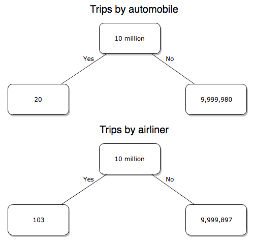
Figure 2. A probability tree to help visualize comparison of deaths (“yes”) by car travel and by airline travel in the United States for the year 2000.
Comparing rates and proportions
Without going into the details, we will do so in Chapter 9 Inferences on Categorical Data, comparing two rates is a chi-square, χ2, contingency table type of problem. More specifically, however, it is a binomial problem (Chapter 3.1, Chapter 6.5); there are two outcomes, death or no death, and we can describe how likely the event is to occur as a proportion. Because the numbers are large, we can use rely on the normal distribution for comparing the two proportions. We’ll explain this more in the next chapters, but for now it may be enough to present the equation for the comparison of two proportions under the assumption of normality, proportion z test.
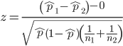
and the null hypothesis (see Chapter 8) tested as that the two proportions are equal. This may be written as
H0 : p1-p2=0
We can assign statistical significance to the differences in events for the two modes of travel under this set of assumptions. Rcmdr has a nice menu-driven system for comparing proportions, but for now I will simply list the R commands.
At the R prompt type each line then submit the command.
total = 100000000
prop.test(c(19700,14),c(total,total)))
And the R output
prop.test(c(19700,14),c(total,total))

    2-sample test for equality of proportions with continuity
    correction

data:  c(19700, 14) out of c(total, total)
X-squared = 19658, df = 1, p-value < 2.2e-16
alternative hypothesis: two.sided
95 percent confidence interval:
 0.0001940984 0.0001996216
sample estimates:
  prop 1   prop 2
1.97e-04 1.40e-07
There’s a bit to unpack here. R is consistent; when it reports results of a statistical test, it typically returns the value of the test statistic (χ2 = 19658), the degrees of freedom for the test (df = 1), and the p-value (< 2.2e-16).
prop.test() were calculated by the Wilson Score method not the Wald method. While both are parametric tests and therefore sensitive to departures from normality (see Chapter 13.3), formulation of Wilson score method makes fewer assumptions (involving approximations of the population proportions) and therefore is considered more accurate.By convention in statistics, if a p-value, where “p” stands for probability, is less than 5%, we would say that our results are statistically significant from the null hypothesis. Looks pretty convincing to me, the difference of 19,700 deaths compared to 14 deaths is clearly different by any criterion and by the results of the statistical test, the p-value is several orders of magnitude smaller than 5%.
Safer to fly. By far, not even close. And similar conclusions would be reached if we compare different years, or averages over many years, or if we used a different way to express the amount of travel (eg, miles/year) by these modes of transportation.
Are you convinced, really? Is it safer to fly?
Let’s try a little statistical reasoning — what assumptions did I make to do these calculations? We recognize immediately that many more people travel by car: that there are way more cars being driven then there are airline planes being flown. The question then is, have we properly adjusted for this difference? Here are a few considerations. My source for the numbers is the NTS 2001 book published by the U.S. Department of Transportation (U.S. Department of Transportation). We are conducting a risk analysis, and the first step is to make sure that we are comparing “apples with apples.” Here are two alternative solutions that at least compare, “Red Delicious” apples with “Macintosh” apples.
Option 1. There are many, many more licensed drivers than there are licensed commercial airline pilots. The standard comparison offered in the background above compared deaths per licensed car driver, but a different metric for air travel, the rate per passenger. This isn’t as bad of a comparison as it may seem — after all, the majority of deaths in car accidents are of the driver themselves. But it isn’t that hard to make the direct comparison — just find out how many commercial pilots there are — a direct comparison with licensed car drivers (stated above as 190,625,023). From the FAA we see that in 2009 there were 125,738 persons with commercial certificates. Since there are only 20 major airline carriers in the United States now (a few more were active in 2000, but we’ll put this aside), the number of licenses is an over estimate of the actual number we want — how many pilots of commercial airlines — but lets use this number for starters — after all, just because a person has a drivers license doesn’t mean they drive or ride in a car.
Number of deaths/yr: Let’s use 2000 data, a typical year prior to 9/11 (and excluding the Covid-19 pandemic). Airlines: 92 deaths; motor vehicles (includes passenger cars, trucks, etc, but not motorcycles): 37,526 deaths (drivers = 25,567; passengers = 10,695; 86 others).
Which mode of travel is riskier? I get a rate a rate of 7.3 X 10⁻⁴ deaths per commercial pilot, or
92125738
compared to a rate for car drivers of 1.97 X 10⁻⁴ deaths.
To summarize what we have so far, I get a result that suggests car travel is almost four times safer
7.3 x 10-41.97 x 10-4→7.31.97 = 3.7
then traveling by commercial airliner. In whole numbers, these results translate to seven deaths for every 10,000 commercial pilots compared to two deaths for every 10,000 licensed car drivers (Fig 3).
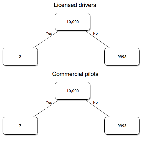
Figure 3. Comparing totals of deaths adjusted by numbers of licensed drivers and by licensed commercial airline pilots in the United States.
R work follows. Enter and submit each command on a separate line in the script window
total = 10000
prop.test(c(2,7),c(total,total))
And the R output
prop.test(c(2,7),c(total,total))

    2-sample test for equality of proportions with continuity
    correction

data:  c(2, 7) out of c(total, total)
X-squared = 1.7786, df = 1, p-value = 0.1823
alternative hypothesis: two.sided
95 percent confidence interval:
 -0.001187816  0.000187816
sample estimates:
prop 1 prop 2
 2e-04  7e-04
What’s happened? The p-value (0.1823) is not less than 5% and so we would conclude under this scenario that there is no difference between the proportions of deaths between the two modes of travel. Let’s keep going.
Option 2. There are many, many more cars on the road then there are airplanes flying commercial passengers. The standard comparison offered in the background information above identified death rates per individual driver, but used a different metric for airline travelers (number of deaths per passenger), which confuses individuals with travelers: what we need is the number of individuals that traveled by airliner, not the total number of passengers (which is many times higher, because of repeat flyers). How can we make a fair comparison for the two modes of travel? Most people never fly whereas most people drive (or ride in a car) frequently in the United States. To me, risk of travel might be better expressed in terms of a per trip rate. I want to know, what are my chances of dying each time I get into my car versus each time I fly on a commercial jet in the United States?
Number of trips/yr. For airlines, I use the number of departures (2000 = 8,951,773). But for cars, we need to decide how to get a similar number. It’s not available directly from the DOT (and would be difficult to get — studies with randomly selected drivers can yield as many as 5 trips per day for licensed drivers). I took the number of licensed drivers and bound the problem — at the low end, let’s say that only 2 trips per week (eg, 50 weeks) are taken by licensed drivers (100 trips); at the upper end, let’s take 2 trips per day per week, or 500 trips/year. Thus, at the low end, we have 1.91 X10¹⁰ trips per year; at the upper end, 9.53 X 10¹⁰ trips per year.
Which mode of travel is riskier? Using the number of deaths/yr listed above in Option 1, I get a rate of 1.03 X 10⁻⁵ deaths/trip for air carriers
928.95 x 10⁶
compared to a rate of 1.97 X 10⁻⁶ deaths/trip for cars (lower bound) or 3.9 X 10⁻⁷ deaths/trip for cars (upper bound). Here’s what the numbers look for in a tree (taking the lower number of trips per year for cars, Fig 4).
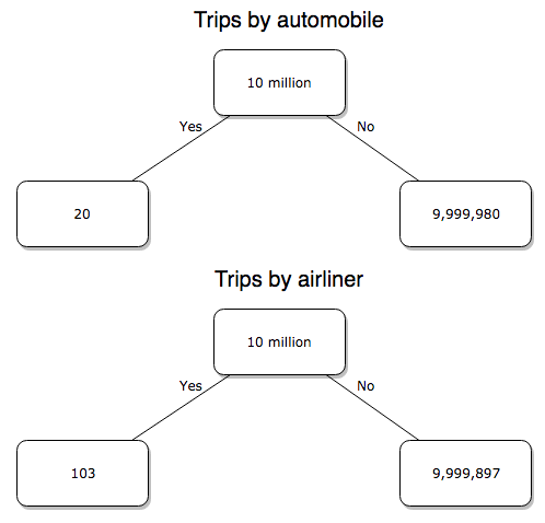
Figure 4. Comparing totals of deaths adjusted by numbers of car trips and by numbers of airline trips in the United States.
R work follow
total = 10000000
prop.test(c(20,103),c(total,total))
And the R output
prop.test(c(20,103),c(total,total))

    2-sample test for equality of proportions with continuity
    correction

data:  c(20, 103) out of c(total, total)
X-squared = 54.667, df = 1, p-value = 1.428e-13
alternative hypothesis: two.sided
95 percent confidence interval:
 -1.057370e-05 -6.026305e-06
sample estimates:
  prop 1   prop 2
2.00e-06 1.03e-05
Now we have another really small p-value (1.428e-13), which suggests a statistically significant difference between the modes of air travel, but the difference in deaths is switched. I now have a result that suggests car travel is much safer than traveling with a commercial airliner! These calculations suggest that you are as much as 26 (upper bounds, five times for lower bounds) times more likely to die from a plane crash then you are behind the wheel. In whole numbers, these results indicate one death for every 100,000 airline flights compared to 1 death for every 500,000 (lower estimate) or 2,500,000 car trips!
Do I have it right and the standard answer is wrong? As Lee Corso used to say on ESPN’s College GameDay program, “Not so fast, my friend!” (Wikipedia). Mark Twain was right to hold the skeptic’s view. Begin by listing the assumptions and by checking the logic of the comparisons (there are still holes in my logic!!). For one, if I am considering my risk of dying by mode of travel, it is far more likely that I will be in a car accident than I will an airline accident, simply because I don’t travel by airline that much. When we consider lifetime risk, we can see why the assertion that it is “safer to fly than drive” is true — we’re far more likely to belong to one of the reference populations involving automobiles (eg, those who drive frequently, for many years) than we are to be among the frequent flyers reference populations.
Questions
1. Review and provide your own examples for
- index
- rate
- ratio
- proportion
3. Like travel safety, we are often confronted by risk comparisons like the following: Which animal is more deadly to humans, dogs or sharks? Between the two, which lead to more hospitalizations in the United States? Work through your assumptions and use results from the International Shark Attack file.
- If a person lives in Nebraska, and never visits the ocean, how does a “shark attack” risk analysis apply? Is it a fair comparison to make between dog attacks and shark attacks? Why or why not.
4. Go to cappex.com/colleges and update institutional (gift) aid offered by Chaminade and HPU. Compare to University of Hawaii-Manoa.
5. Calculate percent increase for
- Annual atmospheric CO2 1980 and 2024.
Quiz Chapter 6.2
Ratios and probabilities
Chapter 6 content
- Introduction
- Some preliminaries
- Ratios and probabilities
- Combinations and permutations
- Types of probability
- Discrete probability distributions
- Continuous distributions
- Normal distribution and the normal deviate (Z)
- Moments
- Chi-square distribution
- t distribution
- F distribution
- References and suggested readings
7.4 – Epidemiology: Relative risk and absolute risk, explained
Risk communication.
Epidemiology is the study of patterns of health and illness of populations. An important task in an epidemiology study is to identify risks associated with disease. Epidemiology is a crucial discipline used to inform about possible effective treatment approaches, health policy, and about the etiology of disease.
Please review terms presented in section 7.1 before proceeding. RR and AR are appropriate for cohort-control and cross-sectional studies (see 2.4 and 5.4) where base rates of exposure and unexposed or numbers of affected and non-affected individuals (prevalence) are available. Calculations of relative risk (RR) and relative risk reduction (RRR) are specific to the sampled groups under study whereas absolute risk (AR) and absolute risk reduction (ARR) pertain to the reference population. Relative risks are specific to the study, absolute risks are generalized to the population. Number needed to treat (NNT) is a way to communicate absolute risk reductions.
An example of ARR and RRR risk calculations using natural numbers.
Clinical trials are perhaps the essential research approach (Sibbald and Roland 1998; Sylvester et al 2017); they are often characterized with a binary outcome. Subjects either get better or they do not. There are many ways to represent risk of a particular outcome, but where possible, using natural numbers is generally preferred as a means of communication, particularly to the general public. Consider the following example (pp 34-35, Gigerenzer 2015): What is the benefit of taking a cholesterol-lowering drug, Pravastatin, on the risk of deaths by heart attacks and other causes of mortality? Press releases (eg, Maugh 1995), from the study stated the following:
“… the drug pravastatin reduced … deaths from all causes 22%”
A subsequent report (Skolbekken 1998) presented the following numbers (Table 1).
Table 1. Reduction in total mortality (5 year study) for people who took Pravastatin compared to those who took placebo.
| Deaths per 1000 people with high cholesterol (> 240 mg/dL) |
No deaths | Cumulative incidence |
||
| Treatment | Pravastatin
(n = 3302) |
a= 32 |
b= 3270 |
CIe |
| Placebo
(n = 3293) |
c= 41 |
d= 3252 |
CIu | |
where cumulative incidence refers to the number of new events or cases of disease divided by the total number of individuals in the population at risk.
Do the calculations of risk
The risk reduction (RR), or the number of people who die without treatment (placebo) minus those who die with treatment (Pravastatin), 
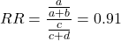
and the cumulative incidence in the exposed (treated) group, CIe, is  , and cumulative incidence in the unexposed (control) group, CIu, is
 . We can calculate another statistic called the risk ratio,
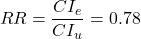
because the risk ratio is less than one, we interpret that statins reduce the risk of mortality from heart attack. In other words, statins lowered the risk by 0.78.
But is this risk reduction meaningful?
Now, consider the absolute risk reduction (ARR) is 
Relative risk reduction, or the absolute risk reduction divided by the proportion of patients who die without treatment, is 
Conclusion: high cholesterol may contribute to increased risk of mortality, but the rate is very low in the population as a whole (the ARR).
Another useful way to communicate benefit is to calculate the Number Needed to Treat (NNT), or the number of people who must receive the treatment to save (benefit) one person. The ideal NNT is a value of one (1), which would be interpreted as everyone improves who receives the treatment. By definition, NNT must be positive; however, a resulting negative NNT would suggest the treatment may cause harm, ie, number needed to harm (NNH).
For this example, the NNT is

therefore, to benefit one person, 111 need to be treated. The flip side of the implications of NNT, although one person may benefit by taking the treatment, 110 ( ) will take the treatment, but will NOT RECEIVE THE BENEFIT, but do potentially get any side effect of the treatment.
Confidence interval for NNT is derived from the Confidence interval for ARR.
For a sample of 100 people drawn at random from a population (which may number in the millions), then repeat the NNT calculation for a different sample of 100 people, do we expect the first and second NNT estimates to be exactly the same number? No, but we do expect them to be close and we can define what we mean by close as we expect each estimate to be within certain limits. While we expect the second calculation to be close to the first estimate, we would be surprised if it was exactly the same. And so, which is the correct estimate, the first or the second? They both are, in the sense that they both estimate the parameter NNT (a property of a population).
We use confidence interval to communicate where we believe the true estimate for NNT to be. Confidence Intervals (CI) allow us to assign a probability to how certain we are about the statistic and whether it is likely to be close to the true value (Altman 1998, Bender 2001). We will calculate the 95% CI for the ARR using the Wald method, then take the inverse of these estimates for our 95% CI. The Wald method assumes normality.
For CI of ARR, we need sample size for control and treatment groups; like all confidence intervals, we need to calculate the standard error of the statistic, in this, case, the standard error (SE) for ARR is approximately

where SE is the standard error for ARR. For our example, we have

The 95% CI for ARR is approximately 
For the Wald estimate, replace the 2 with  , which comes from the normal table for z at

(why the 2 in the equation? Because it is plus or minus so we divide the frequency 0.95 in half) and for our example, we have 
and the inverse for NNT CI is 
Our example exemplifies the limitation of the Wald approach (cf. Altman 1998): our confidence interval includes zero, and doesn’t even include our best estimate of NNT (111).
Note 1: By now I trust you can see differences for results by direct input of the numbers into R and what you get by the natural numbers approach. In part this is because we round in our natural number calculations — remember, while it makes more sense to communicate about whole numbers (people) and not fractions (fractions of people!), rounding through the calculations adds error to the final value. As long as you know the difference and the relevance between approximate and exact solutions, this shouldn’t cause concern.
Software: epiR.
R has many epidemiology packages, epiR and epitools are two. Most of the code presented stems from epiR.
We need to know about our study design in order to tell the functions which statistics are appropriate to estimate. For 2X2 tables, we will use epi.2by2() command, which allows four kinds of studies (Table 2).
Table 2. The method argument in epi.2by2 chooses how to analyze your data based on your study design.
| Method | Description | Notes |
|---|---|---|
| cohort.count | Use this when you follow a set number of people over time and count how many get sick. | This design directly calculates Relative Risk Reduction (RRR) and Absolute Risk Reduction (ARR) because you track baseline risk over time. |
| cohort.time | Use this when you follow people over time and track exactly how long each person was monitored before getting sick. | This calculates rate reductions instead of ARR or RRR because it deals with person-time data rather than raw counts. |
| case.control | Use this when you start with sick people and healthy people and look backwards at their past exposures. | You cannot calculate ARR or RRR here because you do not know the actual baseline risk of the population. |
| cross.sectional | Use this when you take a snapshot of a population at a single point in time to see who is currently exposed and sick. | This calculates prevalence reductions rather than true ARR or RRR because you are not tracking changes over time. |
For our statin example, the design was prospective cohort (ie, cohort.count in epiR package language), not case-control or cross-sectional (review in Chapter 5.4).
library(epiR)
Table1 <- matrix(c(32,3270,41,3252), 2, 2, byrow=TRUE, dimnames = list(c("Statin", "Placebo"), c("Died", "Lived")))
Table1
        Died Lived
Statin    32  3270
Placebo   41  3252
epi.2by2(Table1, method="cohort.count", outcome = "as.columns")
R output
           Outcome + Outcome - Total           Inc risk *
Exposed +         32      3270  3302 0.97  (0.66 to 1.37)
Exposed -         41      3252  3293 1.25  (0.89 to 1.69)
Total             73      6522  6595 1.11  (0.87 to 1.39)

Point estimates and 95% CIs:
-------------------------------------------------------------------
Inc risk ratio                          0.78 (0.49, 1.23)
Inc odds ratio                          0.78 (0.49, 1.24)
Attrib risk in the exposed *           -0.28 (-0.78, 0.23)
Attrib fraction in the exposed (%)    -28.48 (-103.47, 18.88)
Attrib risk in the population *        -0.14 (-0.59, 0.32)
Attrib fraction in the population (%) -12.48 (-37.60, 8.05)
-------------------------------------------------------------------
Uncorrected chi2 test that OR = 1: chi2(1) = 1.147 Pr>chi2 = 0.284
Fisher exact test that OR = 1: Pr>chi2 = 0.292
Wald confidence limits
CI: confidence interval
* Outcomes per 100 population units
The risk ratio we calculated by hand is shown in green in the R output, along with other useful statistics (see ?epi2x2 for help with these additional terms) not defined in our presentation.
We explain results of chi-square goodness of fit (Ch 9.1) and Fisher exact (Ch 9.5) tests in Chapter 9. Suffice to say here, we interpret the p-value (Pr) = 0.284 and 0.292 to indicate that there is no association between mortality from heart attacks with or without the statin (ie, the Odds Ratio, OR, not statistically different from one).
Wait! Where’s NNT and other results?
Use another command in epiR package, epi.tests(), to determine the specificity, sensitivity, and positive (or negative) predictive value.
epi.tests(Table1)
and R returns
          Outcome + Outcome - Total
Test +           32      3270  3302
Test -           41      3252  3293
Total            73      6522  6595

Point estimates and 95% CIs:
--------------------------------------------------------------
Apparent prevalence *                    0.50 (0.49, 0.51)
True prevalence *                        0.01 (0.01, 0.01)
Sensitivity *                            0.44 (0.32, 0.56)
Specificity *                            0.50 (0.49, 0.51)
Positive predictive value *              0.01 (0.01, 0.01)
Negative predictive value *              0.99 (0.98, 0.99)
Positive likelihood ratio                0.87 (0.67, 1.13)
Negative likelihood ratio                1.13 (0.92, 1.38)
False T+ proportion for true D- *        0.50 (0.49, 0.51)
False T- proportion for true D+ *        0.56 (0.44, 0.68)
False T+ proportion for T+ *             0.99 (0.99, 0.99)
False T- proportion for T- *             0.01 (0.01, 0.02)
Correctly classified proportion *        0.50 (0.49, 0.51)
--------------------------------------------------------------
* Exact CIs
Additional statistics are available by saving the output from epi2x2() or epitests() to an object, then using summary(). For example save output from epi.2by2(Table1, method="cohort.count", outcome = "as.columns") to object myEpi, then
summary(myEpi)
look for NNT in the R output
$massoc.detail$NNT.strata.wald
       est    lower    upper
1 -362.377 -128.038  436.481
Thus, the NNT was 362 (compared to 111 we got by hand) with 95% Confidence interval between -436 and +128 (make it positive because it is a treatment improvement).
Note 2: Strata (L. layers), refer to subgroups, for example, sex or age categories (see discussion in Ch05.4). Our examples here are not presented as subgroup analysis, but epiR reports by name strata.
epiR reports a lot of additional statistics in the output and for clarity, I have not defined each one, just the basic terms we need for BI311. As always, see help pages (eg, ?epi.2x2 or ?epitests)for more information about structure of an R command and the output.
We’re good, but we can work the output to make it more useful to us.
Improve output from epiR.
For starters, if we set interpret=TRUE instead of the default, interpret=FALSE, epiR will return a richer response.
fit <- epi.2by2(dat = as.table(Table1), method = "cohort.count", conf.level = 0.95, units = 100, interpret = TRUE, outcome = "as.columns")
fit
R output. In addition to the table of coefficients (above), interpret=TRUE provides more context, shown below
Measures of association strength:
The outcome incidence risk among the exposed was 0.78 (95% CI 0.49 to 1.23) times less than the outcome incidence risk among the unexposed.

The outcome incidence odds among the exposed was 0.78 (95% CI 0.49 to 1.24) times less than the outcome incidence odds among the unexposed.

Measures of effect in the exposed:
Exposure changed the outcome incidence risk in the exposed by -0.28 (95% CI -0.78 to 0.23) per 100 population units. -28.5% of outcomes in the exposed were attributable to exposure (95% CI -103.5% to 18.9%).

Number needed to treat for benefit (NNTB) and harm (NNTH):
The number needed to treat for one subject to be harmed (NNTH) is 362 (NNTH 128 to infinity to NNTB 436).

Measures of effect in the population:
Exposure changed the outcome incidence risk in the population by -0.14 (95% CI -0.59 to 0.32) per 100 population units. -12.5% of outcomes in the population were attributable to exposure (95% CI -37.6% to 8.1%).
That’s quite a bit. Another trick is to get at the table of results. We install a package called broom, which includes a number of ways to handle output from R functions, including those in the epiR package. Broom takes from the TidyVerse environment; tables are stored as tibbles.
Note 3: A tibble (package tibble) is a modified R data frame optimized for the tidyverse that enforces strict data handling and cleaner console printing. Unlike standard data frames, tibbles refuse to automatically simplify into vectors when sliced or guess column names using partial matching. Because of these intentional design choices, tibbles often don’t play well with R functions not written explicitly with the TidyVerse environment in mind.
To convert a data.frame to a tibble,
my_tibble <- as_tibble(my_dataframe)
To convert a tibble back to a standard data.frame
my_dataframe <- as.data.frame(my_tibble)
library(broom)

# Test statistics
tidy(fit, parameters = "stat")
R output
# A tibble: 3 × 4
term statistic df p.value
<chr> <dbl> <dbl> <dbl>
1 chi2.strata.uncor 1.15 1 0.284
2 chi2.strata.yates 0.909 1 0.340
3 chi2.strata.fisher NA NA 0.292
We can convert the tibbles into our familiar data.frame format, and then select only the statistics we want.
# Measures of association
fitD <- as.data.frame(tidy(fit, parameters = "moa")); fitD
R output, all 15 measures of association!
                  term     estimate     conf.low    conf.high
1       RR.strata.wald    0.7783605    0.4914679   1.23272564
2     RR.strata.taylor    0.7783605    0.4914679   1.23272564
3      RR.strata.score    0.8742994    0.6584540   1.10340173
4       OR.strata.wald    0.7761915    0.4876209   1.23553616
5     OR.strata.cfield    0.7761915           NA           NA
6      OR.strata.score    0.7761915    0.4894450   1.23093168
7        OR.strata.mle    0.7762234    0.4718655   1.26668220
8    ARisk.strata.wald   -0.2759557   -0.7810162   0.22910484
9   ARisk.strata.score   -0.2759557   -0.8000574   0.23482532
10     NNT.strata.wald -362.3770579 -128.0383246 436.48140194
11    NNT.strata.score -362.3770579 -124.9910314 425.84844829
12  AFRisk.strata.wald   -0.2847517   -1.0347210   0.18878949
13  PARisk.strata.wald   -0.1381661   -0.5933541   0.31702189
14  PARisk.strata.piri   -0.1381661   -0.3910629   0.11473067
15 PAFRisk.strata.wald   -0.1248227   -0.3760279   0.08052298
We can call out just the statistics we want from this table by calling to the specific elements in the data.frame (rows, columns).
fitD[c(1,4,7,9,12),]
R output
                 term   estimate   conf.low  conf.high
1      RR.strata.wald  0.7783605  0.4914679  1.2327256
4      OR.strata.wald  0.7761915  0.4876209  1.2355362
7       OR.strata.mle  0.7762234  0.4718655  1.2666822
9  ARisk.strata.score -0.2759557 -0.8000574  0.2348253
12 AFRisk.strata.wald -0.2847517 -1.0347210  0.1887895
Software: epitools.
Another useful R package for epidemiology is epitools, but it comes with it’s own idiosyncrasies. We have introduced the standard 2X2 format, with a, b, c, and d cells defined as in Table 1, above. However, epitools does it differently, and we need to update the matrix. By default, epitools has the unexposed group (control) in the first row and the non-outcome (no disease) is in the first column. To match our a,b,c, and d matrix, use the epitools command to change this arrangement with the rev() argument. Now, the analysis will use the contingency table on the right where the exposed group (treatment) is in the first row and the outcome (disease) is in the first column (h/t M. Bounthavong 2021). Once that’s accomplished, epitools returns what you would expect.
Calculate relative risk
risk1 <- 32 / (3270 + 32)
risk2 <- 41 / (3525 + 41)
risk1 - risk2
and R returns
-0.00180638
odds ratio
library(epitools)
oddsratio.wald(Table1, rev = c("both"))
and R returns
$data
              Outcome
Predictor Disease2 Disease1 Total
 Exposed2      517       36   553
 Exposed1      518       11   529
Total         1035       47  1082

$measure
           odds ratio with 95% C.I.
Predictor   estimate      lower      upper
 Exposed2  1.0000000        NA         NA
 Exposed1  0.3049657 0.1535563  0.6056675

$p.value
two-sided
Predictor  midp.exact  fisher.exact    chi.square
Exposed2           NA            NA            NA
Exposed1 0.0002954494  0.0003001641  0.0003517007
odds ratio highlighted in green.
Software: OpenEpi.
R is fully capable of delivering the calculations you need, but sometimes you just want a quick answer. Online, the OpenEpi tools at https://www.openepi.com/ can be used for homework problems. For example, working with count data in 2 X 2 format, select Counts > 2X2 table from the side menu to bring up the data form (Fig 1).
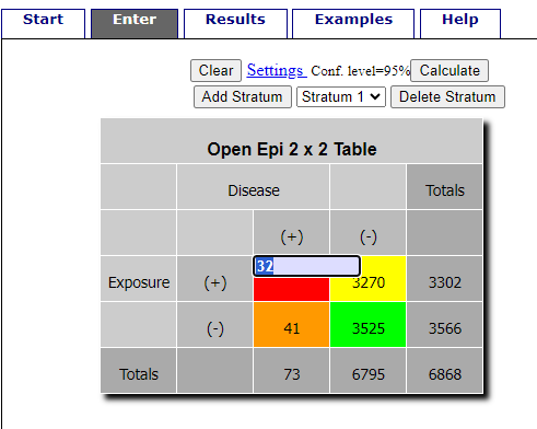
Figure 1. Data entry for 2X2 table at openepi.com.
Once the data are entered, click on the Calculate button to return a suite of results (Fig 2).
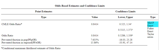
Figure 2. Results for 2X2 table at openepi.com.
Software: RcmdrPlugin.EBM
Note 4: Fall 2023 — I have not been able to run the EBM plugin successfully! The package is still active at CRAN, but looks like it hasn’t been updated since 2015. Simply returns an error message — — on data sets which have in the past performed perfectly. Thus, until further notice, do not use the EBM plugin. Instead, use commands in the epiR package.
This isn’t the place nor can I be the author to discuss what evidence based medicine (EBM) entails (cf. Masic et al. 2008), or what its shortcomings may be (Djulbegovic and Guyatt 2017). Rcmdr has a nice plugin, based on the epiR package, that will calculate ARR, RRR and NNT as well as other statistics. The plugin is called RcmdrPlugin.EBM
install.packages("RcmdrPlugin.EBM", dependencies=TRUE)
After acquiring the package, proceed to install the plug-in. Restart Rcmdr, then select Tools and Rcmdr Plugins (Fig 3).
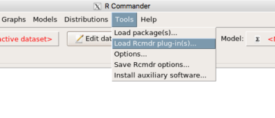
Figure 3. Rcmdr: Tools → Load Rcmdr plugins…
Find the EBM plug-in, then proceed to load the package (Fig 4).
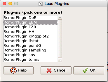
Figure 4. Rcmdr plug-ins available (after first download the files from an R mirror site).
Restart Rcmdr again and the menu “EBM” should be visible in the menu bar. We’re going to enter some data, so choose the Enter two-way table… option in the EBM plug-in (Fig 5)
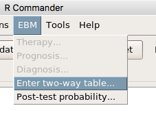
Figure 5. R Commander EBM plug-in, enter 2X2 table menus.
To review, we have the following problem, illustrated with natural numbers and probability tree (Fig 6).
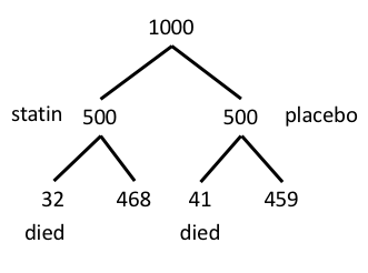
Figure 6. Illustration of probability tree for the statin problem.
Now, let’s enter the data into the EBM plugin. For the data above I entered the counts as
| Lived | Died | |
| Statin | 468 | 32 |
| Placebo | 459 | 41 |
and selected the “Therapy” medical indicator (Fig 7).
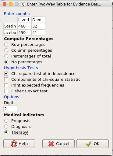
Figure 7. EBM plugin with two-way table completed for the statin problem.
The output from EBM plugin was as follows. I’ve added index numbers in brackets so that we can point to the output that is relevant for our worked example here.
(1) .Table <- matrix(c(468,32,459,41), 2, 2, byrow=TRUE, dimnames = list(c('Drug', 'Placebo'), c('Lived', 'Dead')))
(2) fncEBMCrossTab(.table=.Table, .x='', .y='', .ylab='', .xlab='', .percents='none', .chisq='1', .expected='0', .chisqComp='0', .fisher='0', .indicators='th', .decimals=2)
R output begins by repeating the commands used, here marked by lines (1) and (2). The statistics we want follow in the next several lines of output.
(3) Pearson's Chi-squared test data: .Table X-squared = 1.197, df = 1, p-value = 0.2739
(4) # Notations for calculations Event + Event -Treatment "a" "b" Control "c" "d"
(5)# Absolute risk reduction (ARR) = -1.8 (95% CI -5.02 - 1.42) %. Computed using formula: [c / (c + d)] - [a / (a + b)]
(6)# Relative risk = 1.02 (95% CI 0.98 - 1.06) %. Computed using formula: [c / (c + d)] / [a / (a + b)]
(7)# Odds ratio = 1.31 (95% CI 0.81 - 2.11). Computed using formula: (a / b) / (c / d)
(8) # Number needed to treat = -55.56 (95% CI 70.29 - Inf). Computed using formula: 1 / ARR
9)# Relative risk reduction = -1.96 (95% CI -5.57 - 1.53) %. Computed using formula: { [c / (c + d)] - [a / (a + b)] } / [c / (c + d)]
(10)# To find more about the results, and about how confidence intervals were computed, type ?epi.2by2 . The confidence limits for NNT were computed as 1/ARR confidence limits. The confidence limits for RRR were computed as 1 - RR confidence limits.
end R output
In summary, we found no difference between statin and placebo (P-value = 0.2739) and ARR of -1.8%
Questions.
Data from a case-control study on alcohol use and esophageal cancer (Tuyns et al (1977), example from Gerstman 2014). Cases were men diagnosed with esophageal cancer from a region in France. Controls were selected at random from electoral lists from the same geographical region.
| Esophageal cancer | |||
|
Alcohol grams/day |
Cases | Noncases |
Total |
| > 80 | 96 | 109 |
205 |
|
< 80 |
104 |
666 |
770 |
| Total | 200 | 775 | 975 |
- What was the null hypothesis? Be able to write the hypothesis in symbolic form and as a single sentence.
- What was the alternative hypothesis? Be able to write the hypothesis in symbolic form and as a single sentence.
- What was the observed frequency of subjects with esophageal cancer in this study? And the observed frequency of subjects without esophageal cancer?
- Estimate Relative Risk, Absolute Risk, NNT, and Odds ratio?
- Which is more appropriate, RR or OR? Justify your decision.
- The American College of Obstetricians and Gynecologists recommends that women with an average risk of breast cancer (BC) over 40 get an annual mammogram. Nationally, the sensitivity of mammography is about 68% and specificity of mammography is about 75%. Moreover, mammography involves exposure of women to radiation, which is known to cause mutations. Given that the prevalence of BC in women between 40 and 49 is about 0.1%, please evaluate the value of this recommendation by completing your analysis.
A) In this age group, how many women are expected to develop BC?
B) How many False negative would we expect?
C) How many positive mammograms are likely to be true positives? - “Less than 5% of women with screen-detectable cancers have their lives saved,” (quote from BMC Med Inform Decis Mak. 2009 Apr 2;9:18. doi: 10.1186/1472-6947-9-18): Using the information from question 5, What is the Number Needed to Treat for mammography screening?
Quiz Chapter 7.4
Epidemiology: Relative risk and absolute risk, explained
Chapter 7 contents
- Probability, Risk Analysis
- Epidemiology definitions
- Epidemiology basics
- Conditional Probability and Evidence Based Medicine
- Epidemiology: Relative risk and absolute risk, explained
- Odds ratio
- Confidence intervals
- References and suggested readings
7.3 – Conditional Probability and Evidence Based Medicine
- Conditional probability and risk communication
- Probability and independent events
- Example of multiple, independent events
- Probabilistic risk analysis
- Conditional probability of non-independent events
- Diagnosis from testing
- Standard million
- Per capita rate
- Practice and introduce PPV and test decision criteria
- Evidence Based Medicine
- Software
- Example
- Questions
- Quiz
- Chapter 7 contents
Conditional probability and risk communication.
Conditional probabilities can be used to accurately and effectively convey the risk of specific health outcomes to patients and the public. Tools introduced in this chapter help move from an initial assessment of disease risk to a revised probability after a test result is returned. Although there are other interpretations, here we frame EBM — evidence-based-medicine — as a form of Bayesian decision-making.
This sub-chapter covers a lot of ground. We begin by addressing how probability of multiple events are calculated assuming each event is independent. The assumption of independence is then relaxed, and how to determine probability of an event happening given another event has already occurred, conditional probability, is introduced. Use of conditional probability to interpret results of a clinical test are also introduced, along with the concept of EBM. We also introduce Bayes’ rule and Bayesian probability.
Probability and independent events.
Probability distributions are mathematical descriptions of the probabilities of how often different possible outcomes occur. We also introduced basic concepts related to working with the probabilities involving more than one event.
For review, for independent events, you multiply the individual chance that each event occurs to get the overall probability.
Example of multiple, independent events.
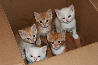
Figure 1. Now that’s a box full of kittens. Creative Commons License, source: https://www.flickr.com/photos/83014408@N00/160490011.
What is the chance of five kittens in a litter of five to be of the same sex? In feral cat colonies, siblings in a litter share the same mother, but not necessarily the same father, superfecundation. Singleton births are independent events, thus the probability of the first kitten is female is 50%; the second kitten is female, also 50%; and so on. We can multiply the independent probabilities (hence, the multiplicative rule), to get our answer:
kittens <- c(0.5, 0.5, 0.5, 0.5, 0.5)
prod(kittens)
[1] 0.03125
Probabilistic risk analysis.
Risk analysis is the use of information to identify hazards and to estimate the risk. A more serious example. Consider the 1986 Space Shuttle Challenger Disaster (Hastings 2003). Among the crew killed was Ellison Onizuka, the first Asian American to fly in space (Fig 2, first on left back row). Onizuka was born and raised on Hawai`i and graduated from Konawaena High School in 1964.

Figure 2. STS-51-L crew: (front row) Michael J. Smith, Dick Scobee, Ronald McNair; (back row) Ellison Onizuka, Christa McAuliffe, Gregory Jarvis, Judith Resnik. Image by NASA – NASA Human Space Flight Gallery, Public Domain.
The shuttle was destroyed just 73 seconds after lift off (Fig 3).

Figure 3. Space Shuttle Challenger launches from launchpad 39B Kennedy Space Center, FL, at the start of STS-51-L. Hundreds of shorebirds in flight. Image by NASA – NASA Human Space Flight Gallery, Public Domain.
This next section relies on material and analysis presented in the Rogers Commission Report June 1986. NASA had estimated that the probability of one engine failure would be 1 in 100 or 0.01; two engine failures would mean the shuttle would be lost. Thus, the probability of two rockets failing at the same time was calculated as 0.01 X 0.01, which is 0.0001 or 0.01%.
NASA had planned to fly the fleet of shuttles 100 times per year, which would translate to a shuttle failure once in 100 years. The Challenger launch on January 28, 1986, represented only the 25th flight of the shuttle fleet.
One difference on launch day was that the air temperature at Cape Canaveral was quite low for that time of year, as low as 22 °F overnight.
Attention was pointed at the large O-rings in the boosters (engines). In all, there were six of these O-rings. Testing suggested that, at the colder air temperatures, the chance that one of the rings would fail was 0.023. Thus, the chance of success was only 0.977. Assuming independence, what is the chance that the shuttle would experience O-ring failure?
shuttle <- c(0.977, 0.977, 0.977, 0.977, 0.977, 0.977)
#probability of success then was
prod(shuttle)
[1] 0.869

#and therefore probability of failure was
1 - prod(shuttle)
[1] 0.1303042
Conditional probability of non-independent events.
But in many other cases, independence of events cannot be assumed. The probability of an event given that another event has occurred is referred to as conditional probability. Conditional probability is used extensively to convey risk. We’ve touched on some of these examples already:
- the risk of subsequent coronary events given high cholesterol;
- the risk of lung cancer given a person smokes tobacco;
- the risk of mortality from breast cancer given that regular mammography screening was conducted.
There are many, many examples in medicine, insurance, you name it. It is even an important concept that judges and lawyers need to be able to handle (eg, discussion in Berry 2008).
A trigger warning: what follows is emotional, traumatic material, provided to emphasize the importance of these concepts, and the far-reaching implications understanding conditional probability can have for us.
A now famous example of conditional probability in the legal arena came from arguments over the chance that a husband or partner who beats his wife will subsequently murder her — this was an argument raised by the prosecution during pre-trial in the 1995 O.J. Simpson trial (The People of the State of California v. Orenthal James Simpson), and successfully argued by O.J. Simpson’s attorneys… judge ruled in favor of the defense and evidence of O.J. Simpson’s prior abuse were not included in trial. Gigerenzer (2002, following discussions by others, eg, Good 1995) and others (eg, Skorupski and Wainer 2015), have called this the Defendent’s Fallacy, the reverse of the Prosecutor’s Fallacy, where the more typical scenario is that the prosecution provides a list of probabilities about characteristics of the defendant, leaving the jury to conclude that no one else could have possibly fit the description ( and 1987).
In the O.J. Simpson case, the argument went something like this. From the CDC we find that the chance of an average woman being murdered by a stranger or an unrelated party was about 1 in 20,000. CDC statistics indicate 1.3 million women are abused each year by their partner or former partner; each year about 1000 women are murdered. One thousand divided by 1.3 million is a small number, so even when there is abuse the argument goes, 99% of the time there is not murder. The Simpson judge ruled in favor of the defense and much of the evidence of prior abuse was excluded.
Something is missing from the defense’s argument. Nicole Brown Simpson did not belong to a population of battered women — she belonged to the population of murdered women. When we ask, if a woman is murdered, what is the chance that she knew her murderer, we find that more than 55% knew their murderer — and of that 55%, 93% were killed by a partner who had a history of prior abuse against the victim.
Instead of looking at all 1.3 million abused women, we isolate a representative cohort of 100,000 abused women to see what mathematically happens to them in a given year:
Group 1: Murdered by their abuser. According to the defense’s rate of 1 in 2,500:
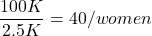
Group 2: Murdered by someone else:
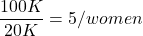
Given that an abused woman was murdered, what is the probability it was done by her abuser?

or 89%.
This is a huge difference from how the Defense portrayed the chance, where they wanted the judge to assume every single one of those 2500 abusers is equally likely to have committed the crime. In reality, we must condition the match on all other available evidence.
The key — Nicole Simpson (and Ron Goldman) were murdered; O.J. Simpson was an ex-partner who had been guilty of assault against Nicole Simpson. Now, it goes from an impossibly small chance, to a much greater chance. Conditional probability, and specifically Bayes’ rule, is used for these kinds of problems. The defense successfully masked a probability that was heavily stacked against their client.
Bayes’ rule provides guidance for how to update the probability of an event based on new evidence. Named after Thomas Bayes (1701- 1761), more generally, Bayes’ rule, described below, is used to quantify conditional probability. Bayesian probability, where probability is interpreted as reasonably expectation instead of frequency of some event. We discuss Bayesian and Frequentist approaches to hypothesis testing in Chapter 8.2.
Note 1: Following our epidemilogy definitions, women murdered by their abuser (Group 2), epidemiology terms, that would be  , the exposure rate in controls, whereas abused woman murdered by her abuser (Group 1), that would be
 , the exposure rate in cases.
Diagnosis from testing.
Let’s turn our attention to medicine. A growing practice in medicine is to claim that decision making in medicine should be based on approaches that give us the best decisions. A search of PubMed texts for “evidence based medicine” found more than 91,944 (13 October 2021, and increase of thirteen thousand since last I looked (10 October, 2019). Evidence based medicine (EBM) is the “conscientious, explicit, judicious and reasonable use of modern, best evidence in making decisions about the care of individual patients” (Masic et al 2008). By evidence, we may mean results from quantitative, systematic reviews, meta-analysis, of research on a topic of medical interest, eg, Cochrane Reviews.
Note 2: Primary research refers to generating or collecting original data in pursuit of tests of hypotheses. Both systematic reviews and meta-analysis are secondary research or “research on research.” As opposed to a literature review, systematic review make explicit how studies were searched for and included; if enough reasonably similar quantitative data are obtained through this process, the reviewer can combine the data and conduct an analysis to assess whether a treatment is effective (De Vries 2018).
As you know, no diagnostic test is 100% fool-proof. For many reasons, test results come back positive when the person truly does not have the condition — this is a false positive result. Correctly identifying individuals who do not have the condition, 100% – false positive rate, is called the specificity of a test.
Think of specificity in this way — provide the test 100 true negative samples (eg, 100 samples from people who do not have cancer) — how many times out of 100 does the test correctly return a “negative”? If 99 times out of 100, then the specificity rate for this test is 99%. Which is pretty good. But the test results mean more if the condition/disease is common; for rare conditions, even 99% is not good enough. Incorrect assignments are rare, we believe, in part because the tests are generally quite accurate. However, what we don’t consider is that detection and diagnosis from tests also depend on the base rate — how frequent the incidence of the condition is in the population. Paradoxically, the lower the base rate, the poorer diagnostic value even a sensitive test may have.
Note 3: This concept, that the base rate effects clinical relevance of interpreting testing — has really important, real-world consequences. It directly bears on clinical testing of cancer and other relatively rare diseases; it also dramatically influences applicability of highly sensitive tests for drug use in clinical samples.
To summarize our jargon for interpreting a test or assay, so far we have
- True positive (a), the person has a disease and the test correctly identifies the person as having the disease.
- False positive (b), test result incorrectly identifies disease; the person does not have the disease, but the test classifies the person as having the disease.
- False negative (c), test result incorrectly classifies person does not have disease, but the person actually has the disease.
- True negative (d), the person does not have the disease and the test correctly categorizes the person as not having the disease.
- Positive predictive value (PPV), the proportion of patients with a positive test result who actually have the disease,
 .
- Negative Predictive Value (NPV), the probability that a person who receives a negative test result really does not have the disease,
 .
- Negative Predictive Value (NPV), the probability that a person who receives a negative test result really does not have the disease,
- Sensitivity of test (Se), the proportion of persons who test positive and do have the disease (true positives):
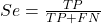
If a test has 75% sensitivity, then out of 100 individuals who do have the disease, then 75 will test positive (TP = true positive). - Specificity of a test (Sp), refers to the rate that a test correctly classifies a person that does not have the disease (TN = true negatives):
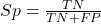
If a test has 90% specificity, then out of 100 individuals who truly do not have the disease, then 90 will test negative (= true negatives).
A worked example. A 50 year old male patient is in the doctor’s office. The doctor is reviewing results from a diagnostic test, eg, a FOBT — fecal occult blood test — a test used as a screening tool for colorectal cancer (CRC). The doctor knows that the test has a sensitivity of about 75% and specificity of about 90%. Prevalence of CRC in this age group is about 0.2% (cf NCI SEER). The prevalence is also the prior probability — the baseline rate of the condition in the population before a test is taken. Figure 4 shows our probability tree using our natural numbers approach (Fig 4).
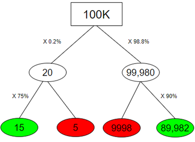
Figure 4. Probability tree for FOBT test; Good test outcomes shown in green: TP stands for true positive and TN stands for true negative. Poor outcomes of a test shown in red: FN stands for false negative and FP stands for false positive.
Note 4: Since U.S. Preventative Task Force (2021), FOBT has largely been replaced by Fecal Immunochemical Test (FIT): sensitivity 74%, specificity 95%, and Multitarget Stool DNA Test: sensitivity 76%, specificity 90%. Cologuard combines both: sensitivity 92%, specificity 97% (cf discussion in Imperiale et al 2014).
- The U.S. Supreme Court (Kennedy v. Braidwood Management, Inc) supported USPSTF’s authority to recommend preventive services covered by insurers (see 2025 article by R. Payerchin in Medical Economics).
The associated probabilities for the four possible outcomes of these kinds of tests (eg, what’s the probability of a person who has tested positive in screening tests actually has the disease?) are shown in Table 1.
Table 1. A 2 X 2 table of possible outcomes of a diagnostic test.
| Person really has the disease | ||
| Test Result | Yes | No |
| Positive | a TP |
b FP |
| Negative | c FN |
d TN |
We want the posterior probability — the chance that a positive test result is a true positive. Bayes’ rule is often given in probabilities,

Bayes’ rule, where truth is represented by either D (the person really does have the disease”) or ND (the person really does not have the disease”) and ⊕ is symbol for “exclusive or” and reads “not D” in this example.
An easier way to see this is to use frequencies and our table instead (Table 1, numbers in Figure 4).
Now, the formula is

Simplified Bayes’ rule, where a is the number of people who test positive and DO HAVE the disease and b is the number of people who test positive and DO NOT have the disease. Thus,  , the posterior probability was

or 0.15%. Because the condition is so rare (0.2% prior) and the test generates a very high number of False Positives (9,998), getting a positive result actually lowers oour confidence slightly from the base rate (from 0.2% down to 0.15%). This occurs because the test is highly unreliable in screening this specific population — it’s known as the base rate fallacy. Thus, the chance that a positive FOBT test for our 50 year old male patient is 99.85% likely wrong.
Standardized million.
Where did the 100,000 come from? We discussed this in chapter 2: it’s a simple trick to adjust rates to the same population size. We use this to work with natural numbers instead of percent or frequencies. You choose to correct to a standardized population based on the raw incidence rate. A rough rule of thumb:
Table 2. Relationship between standard population size and incidence rate.
| Raw IR rate about | IR | Standard population |
| 1/10 | 10% | 1000 |
| 1/100 | 1% | 10,000 |
| 1/1000 | 0.1% | 100,000 |
| 1/10,000 | 0.01% | 1,000,000 |
| 1/100,000 | 0.001% | 10,000,000 |
| 1/1,000,000 | 0.0001% | 100,000,000 |
The raw incident rate is simply the number of new cases divided by the total population.
Per capita rate.
Yet another standard manipulation is to consider the average incidence per person, or per capita rate. The Latin “per capita” translates to “by head” (Google translate), but in economics, epidemiology, and other fields it is used to reflect rates per person. Tuberculosis is a serious infectious disease of primarily the lungs. Incidence rates of tuberculosis in the United States have trended down since the mid 1900s: 52.6 per 100K in 1953 to 2.7 per 100K in 2019 (CDC). Corresponding per capita values are 5.26 x 10⁻⁴ and 2.7 x 10⁻⁵, respectively. Divide the rate by 100,000 to get per person rate.
Practice and introduce PPV and test decision criteria.
Let’s break these problems down, and in doing so, introduce some terminology common to the field of “risk analysis” as it pertains to evaluating assay and diagnotistc tests in biology and epidemiology. Our first example considers the fecal occult blood test, FOBT, test. Blood in the stool may (or may not) indicate polys or colon cancer (Park et al 2010).
A table like the one shown above (Table 1) will appear again and again throughout this and subsequent chapters, but in different forms. We start with Table 3.
Table 3. A 2 X 2 table of possible outcomes of FOBT test.
| Person really has the disease | |||
| Yes | No | ||
| Positive | 15 | 9998 | PPV = 15/(15+9998) = 0.15% |
| Negative | 5 | 89,982 | NPV = 89982/(89982+5) = 99.99% |
We want to know how good is the test, particularly if the goal is early detection? This is conveyed by the PPV, positive predictive value of the test. Unfortunately, the prevalence of a condition is also at play: the lower the prevalence, the lower the PPV must be, because most positive tests will be false when population prevalence is low.
Youden (1950) proposed a now widely adopted index that summarizes how effective a test is. Youden’s J is the sum of specificity and sensitivity minus one.

where Se stands for sensitivity of the test and Sp stands for sensitivity of the test.
Youden’s J takes on values between 0, for a terrible test, and 1, for a perfect test. For our FOBT example, Youden’s J was 0.65. This statistic looks like it’s independent of prevalence, but it’s use as a decision criterion (eg, a cutoff value, above which test is positive, below test is considered negative), assumes that the cost of misclassification (false positives, false negatives) are equal. Prevalence affects number of false positives and false negatives for a given diagnostic test, so any decision criterion based on Youden’s J will also be influenced by prevalence (Smits 2010).
Youden’s J is insensitive to base rates and therefore may be of little practical use in the field. Unsurprisingly, other tools are available, including Matthew’s Correlation Coefficient (MCC),

and the positive and negtive Clinical Utility Index (CUI+, CUI-),

or the F1-score,

epiR will calculate Youden’s J, but the others are either calculated by hand or by way of additional packages. So, we’ll provide a function.
R code to calculate testing decision criteria — code genereated with Gemini AI assistance.
run_screening_wizard <- function() {
# 1. Sequential user prompts starting with cell a
cat("--- 2x2 Matrix Entry Wizard ---\n")
a <- as.numeric(readline(prompt = "Enter cell a (True Positives, TP): "))
b <- as.numeric(readline(prompt = "Enter cell b (False Positives, FP): "))
c <- as.numeric(readline(prompt = "Enter cell c (False Negatives, FN): "))
d <- as.numeric(readline(prompt = "Enter cell d (True Negatives, TN): "))

# 2. Map cells to short variables for calculation
tp <- a
fp <- b
fn <- c
tn <- d

# 3. Construct and print the visual 2x2 matrix
user_matrix <- matrix(
c(tp, fp, fn, tn),
nrow = 2,
byrow = TRUE,
dimnames = list(Test = c("+", "-"), Disease = c("+", "-"))
)
cat("\n[+] Captured Matrix:\n")
print(user_matrix)

# 4. Run background metrics math
sensitivity <- tp / (tp + fn)
specificity <- tn / (tn + fp)
ppv <- tp / (tp + fp)
if (is.nan(ppv)) ppv <- 0

youden_j <- sensitivity + specificity - 1
cui_pos <- sensitivity * ppv

f1_score <- 2 * ((ppv * sensitivity) / (ppv + sensitivity))
if (is.nan(f1_score)) f1_score <- 0

mcc_num <- (tp * tn) - (fp * fn)
mcc_den <- sqrt(as.numeric(tp + fp) * as.numeric(tp + fn) *
as.numeric(tn + fp) * as.numeric(tn + fn))
mcc <- if (mcc_den == 0) 0 else mcc_num / mcc_den

# 5. Compile into the copy/paste ready console matrix
output_matrix <- matrix(
c(round(youden_j, 4), "No", "Good (Overly optimistic baseline)",
round(mcc, 4), "Yes", "Poor (Correctly captures imbalance)",
round(cui_pos, 4), "Yes", "Unacceptable clinical utility",
round(f1_score, 4), "Yes", "Near-total prediction failure"),
nrow = 4, byrow = TRUE
)

dimnames(output_matrix) <- list(
c("Youden's J Index", "MCC", "CUI+", "F1-Score"),
c("Value", "Base_Rate_Dep", "Console_Interpretation")
)

final_df <- as.data.frame(output_matrix)

# 6. Print and invisibly return the dataframe
cat("\n[+] Resulting Metrics Table (Copy/Paste Ready):\n")
print(final_df)
return(invisible(final_df))
}

# Run the function at the R command prompt.
run_screening_wizard()
End R code.
Thus, using a metric sensitive to low base rate, our FOBT tests are (modified from R output)
Table 4. Decision criteria.
| Value | Base rate dependent? | Interpretation | |
 |
0.65 | No | Good |
 |
0.0306 | Yes | Poor |
 |
0.0011 | Yes | Unacceptable clinical utility |
 |
0.0030 | Yes | Near-total prediction failure |
Another worked example. A study on cholesterol-lowering drugs (statins) reported a relative risk reduction of death from cardiac event by 22%. This does not mean that for every 1000 people fitting the population studied, 220 people would be spared from having a heart attack. In the study, the death rate per 1000 people was 32 for the statin versus 41 for the placebo — recall that a placebo is a control treatment offered to overcome potential patient psychological bias (see Chapter 5.4). The absolute risk reduction due to statin is only 41 – 32 or 9 in 1000 or 0.9%. By contrast, relative risk reduction is calculated as the ratio of the absolute risk reduction (9) divided by the proportion of patients who died without treatment (41), which is 22% (LIPID Study Group 1998).
Note that risk reduction is often conveyed as a relative rather than as an absolute number. The distinction is important for understanding arguments based in conditional probability. Thus, the question we want to ask about a test is summarized by absolute risk reduction (ARR) and number needed to treat (NNT), and for problems that include control subjects, relative risk reduction (RRR). We expand on these topics in the next section, 7.4 – Epidemiology: Relative risk and absolute risk, explained.
Evidence Based Medicine.
One culture change in medicine is the explicit intent to make decisions based on evidence (Masic et al 2008). Of course, the joke then is, well, what were doctors doing before, diagnosing without evidence? The comic strip xkcd offers one possible answer (Fig 5).
Figure 5. A summary of “evidence based medical” decisions, perhaps? “Watson Medical Algorithm,” https://xkcd.com/1619/.
As you can imagine, there’s considerable reflection about the EBM movement (see discussions in response to Accad and Francis 2018, eg, Goh 2018). More practically, our objective is for you to be able to work your way through word problems involving risk analysis. You can expect to be asked to calculate, or at least set up for calculation, any of the statistics listed above (eg, False negative, false positive, etc.). Practice problems are listed at the end of this section, and additional problems are provided to you (Homework 4). You’ll also want to check your work, and in any real analysis, you’d most likely want to use R.
Software.
R has several epidemiology packages, and with some effort, can save you time. Another option is to run your problems in OpenEpi, a browser-based set of tools. OpenEpi is discussed with examples in the next section, 7.4.
Here, we illustrate some capabilities of the epiR package, expanded more also in the next section, 7.4. We’ll use the example from Table 3.
R code
library(epiR)
Table3 <- matrix(c(15, 5, 9998, 89982), nrow = 2, ncol = 2)
epi.tests(Table3)
R output
         Outcome + Outcome -   Total
Test +          15      9998   10013
Test -           5     89982   89987
Total           20     99980  100000

Point estimates and 95% CIs:
--------------------------------------------------------------
Apparent prevalence *                      0.10 (0.10, 0.10)
True prevalence *                          0.00 (0.00, 0.00)
Sensitivity *                              0.75 (0.51, 0.91)
Specificity *                              0.90 (0.90, 0.90)
Positive predictive value *                0.00 (0.00, 0.00)
Negative predictive value *                1.00 (1.00, 1.00)
Positive likelihood ratio                  7.50 (5.82, 9.67)
Negative likelihood ratio                  0.28 (0.13, 0.59)
False T+ proportion for true D- *          0.10 (0.10, 0.10)
False T- proportion for true D+ *          0.25 (0.09, 0.49)
False T+ proportion for T+ *               1.00 (1.00, 1.00)
False T- proportion for T- *               0.00 (0.00, 0.00)
Correctly classified proportion *          0.90 (0.90, 0.90)
--------------------------------------------------------------
* Exact CIs
Oops! I wanted PPV, which by hand calculation was 0.15%, but R reported “0.00?” This is a significant figure reporting issue. The simplest solution is to submit options(digits=6) before the command, then save the output from epi.tests() to an object and use summary(). For example
options(digits=6)
myEpi <- epi.tests(Table3)
summary(myEpi)
And R returns
     statistic           est        lower        upper
1           ap  0.1001300000 0.0982761568  0.102007072
2           tp  0.0002000000 0.0001221693  0.000308867
3           se  0.7500000000 0.5089541283  0.913428531
4           sp  0.9000000000 0.8981238085  0.901852950
5      diag.ac  0.8999700000 0.8980937508  0.901823014
6      diag.or 27.0000000000 9.8110071871 74.304297826
7         nndx  1.5384615385 1.2265702376  2.456532054
8       youden  0.6500000000 0.4070779368  0.815281481
9       pv.pos  0.0014980525 0.0008386834  0.002469608
10      pv.neg  0.9999444364 0.9998703379  0.999981958
11      lr.pos  7.5000000000 5.8193604069  9.666010707
12      lr.neg  0.2777777778 0.1300251423  0.593427490
13      p.rout  0.8998700000 0.8979929278  0.901723843
14       p.rin  0.1001300000 0.0982761568  0.102007072
15      p.tpdn  0.1000000000 0.0981470498  0.101876192
16      p.tndp  0.2500000000 0.0865714691  0.491045872
17      p.dntp  0.9985019475 0.9975303919  0.999161317
18      p.dptn  0.0000555636 0.0000180416  0.000129662
There we go — pv.pos reported as 0.0014980525, which, after turning to a percent and rounding, we have 0.15%. Note also the additional statistics provided — a good rule of thumb — always try to save the output to an object, then view the object, eg, with summary(). Refer to help pages for additional details of the output (?epi.tests).
What about R Commander menus?
Note 3: Confirmed Fall 2026 — I have not been able to run the EBM plugin successfully! Simply returns an error message — — on data sets which have in the past performed perfectly. Thus, until further notice, do not use the EBM plugin. Instead, use commands in the epiR package. I’m leaving the text here on the chance the error with the plugin is fixed.
Rcmdr has a plugin that will calculate ARR, RRR and NNT. The plugin is called RcmdrPlugin.EBM (Leucuta et al 2014) and it would be downloaded as for any other package via R.
Download the package from your selected R mirror site, then start R Commander.
install.packages("RcmdrPlugin.EBM")
From within R Commander (Fig 6), select
Tools → Load Rcmdr plug-in(s)…
Figure 6. To install an Rcmdr plugin, first go to Rcmdr → Tools → Load Rcmdr plug-in(s)…
Next, select from the list the plug-in you want to load into memory, in this case, RcmdrPlugin.EBM (Fig 7).
Figure 7. Select the Rcmdr plugin, then click the “OK” button to proceed.
Restart Rcmdr again (Fig 8),
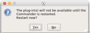
Figure 8. Select “Yes” to restart R Commander and finish installation of the plug-in.
and the menu “EBM” should be visible in the menu bar (Fig 9).
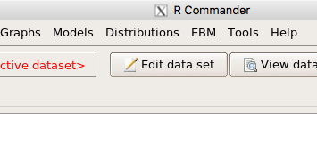
Figure 9. After restart of R Commander the EBM plug-in is now visible in the menu.
Note that you will need to repeat these steps each time you wish to work with a plug-in, unless you modify your .RProfile file. See
Rcmdr → Tools → Save Rcmdr options…
Clicking on the EBM menu item brings up the template for the Evidence Based Medicine module. We’ll mostly work with 2 X 2 tables (eg, see Table 1) , so select the “Enter two-way table…” option to proceed (Fig 10).
Figure 10. Select “Enter two-way table…”.
And finally, Figure 11 shows the two-way table entry cells along with options. We’ll try a problem by hand then use the EBM plugin to confirm and gain additional insight.
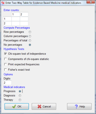
Figure 11. Two-way table Rcmdr EBM plug-in.
For assessing how good a test or assay is, use the Diagnosis option in the EBM plugin. For situations with treated and control groups, use Therapy option. For situations in which you are comparing exposure groups (eg, smokers vs non-smokers), use the Prognosis option.
Example.
Here’s a simple one (problem from Gigerenzer 2002).
About 0.01% of men in Germany with no known risk factors are currently infected with HIV. If a man from this population actually has the disease, there is a 99.9% chance the tests will be positive. If a man from this population is not infected, there is a 99.9% chance that the test will be negative. What is the chance that a man who tests positive actually has the disease?
Start with the reference, or base population (Figure 12). It’s easy to determine the rate of HIV infection in the population if you use numbers. For 10,000 men in this group, exactly one man is likely to have HIV (0.0001X10,000), whereas 9,999 would not be infected.
For the man who has the disease it’s virtually certain that his results will be positive for the virus (because the sensitivity rate = 99.9%). For the other 9,999 men, one will test positive (the false positive rate = 1 – specificity rate = 0.01%).
Thus, for this population of men, for every two who test positive, one has the disease and one does not, so the probability even given a positive test is only 100*1/2 = 50%. This would also be the test’s Positive Predictive Value.
Note that if the base rate changes, then the final answer changes! For example, if the base rate was 10%
It also helps to draw a tree to help you determine the numbers (Fig 12)
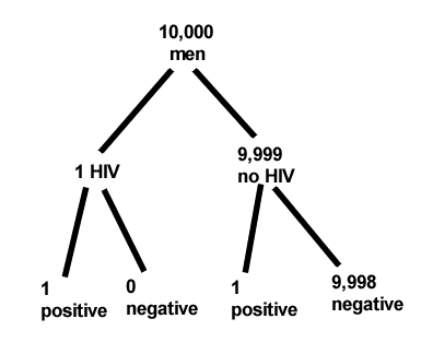
Figure 12. Draw a probability tree to help with the frequencies.
From our probability tree in Figure 12 it is straight-forward to collect the information we need.
- Given this population, how many are expected to have HIV? Two.
- Given the specificity and sensitivity of the assay for HIV, how many persons from this population will test positive? Two.
- For every positive test result, how many men from this population will actually have HIV? One.
Thus, given this population with the known risk associated, the probability that a man testing positive actually has HIV is 50% (=1/(1+1)).
Use the EBM plugin. Select two-way table, then enter the values as shown in Fig 13.
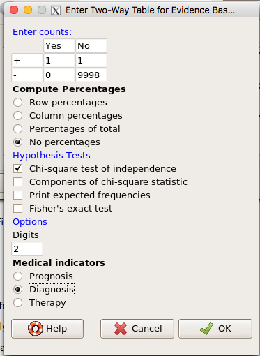
Figure 13. EBM plugin with data entry.
Select the “Diagnosis” option — we are answering the question: How probable is a positive result given information about sensitivity and specificity of a diagnosis test. The results from the EBM functions are given below
Rcmdr> .Table
      Yes No
   +  1    1
   -  0 9998
Rcmdr> fncEBMCrossTab(.table=.Table, .x='', .y='', .ylab='', .xlab='',
Rcmdr+ .percents='none', .chisq='1', .expected='0', .chisqComp='0', .fisher='0',
Rcmdr+ .indicators='dg', .decimals=2)
# Notations for calculations
        Disease + Disease -
Test +      "a"         "b"
Test -      "c"         "d"
# Sensitivity (Se) = 100 (95% CI 2.5 - 100) %. Computed using formula: a / (a + c)
# Specificity (Sp) = 99.99 (95% CI 99.94 - 100) %. Computed using formula: d / (b + d)
# Diagnostic accuracy (% of all correct results) = 99.99 (95% CI 99.94 - 100) %. Computed using formula: (a + d) / (a + b + c + d)
# Youden's index = 1 (95% CI 0.02 - 1). Computed using formula: Se + Sp - 1
# Likelihood ratio of a positive test = 9999 (95% CI 1408.63 - 70976.66). Computed using formula: Se / (Sp - 1)
# Likelihood ratio of a negative test = 0 (95% CI 0 - NaN). Computed using formula: (1 - Se) / Sp
# Positive predictive value = 50 (95% CI 1.26 - 98.74) %. Computed using formula: a / (a + b)
# Negative predictive value = 100 (95% CI 99.96 - 100) %. Computed using formula: d / (c + d)
# Number needed to diagnose = 1 (95% CI 1 - 40.91). Computed using formula: 1 / [Se - (1 - Sp)]
Note that the formulas used to calculate Sensitivity, Specificity, etc., follow our Table 1 (compare to “Notations for calculations”). The use of EBM provides calculations of our confidence intervals.
Questions.
- The sensitivity of the fecal occult blood test (FOBT) is reported to be 0.68. What is the False Negative Rate?
- The specificity of the fecal occult blood test (FOBT) is reported to be 0.98. What is the False Positive Rate?
- For men between 50 and 54 years of age, the rate of colon cancer is 61 per 100,000. If the false negative rate of the fecal occult blood test (FOBT) is 10%, how many persons who have colon cancer will test negative?
- For men between 50 and 54 years of age, the rate of colon cancer is 61 per 100,000. If the false positive rate of the fecal occult blood test (FOBT) is 10%, how many persons who do not have colon cancer will test positive?
- A study was conducted to see if mammograms reduced mortality
Mammogram Deaths/1000 women No 4 Yes 3 data from Table 5-1 p. 60 Gigerenzer (2002)
What is the RRR? - A study was conducted to see if mammograms reduced mortality
Mammogram Deaths/1000 women No 4 Yes 3 data from Table 5-1 p. 60 Gigerenzer (2002)
What is the NNT? - Does supplemental Vitamin C decrease risk of stroke in Type II diabetic women? A study conducted on 1923 women, a total of 57 women had a stroke, 14 in the normal Vitamin C level and 32 in the high Vitamin C level. What is the NNT between normal and high supplemental Vitamin C groups?
- Sensitivity of a test is defined as
A. False Positive Rate
B. True Positive Rate
C. False Negative Rate
D. True Negative Rate - Specificity of a test is defined as
A. False Positive Rate
B. True Positive Rate
C. False Negative Rate
D. True Negative Rate - In thinking about the results of a test of a null hypothesis, Type I error rate is equivalent to
A. False Positive Rate
B. True Positive Rate
C. False Negative Rate
D. True Negative Rate - During the Covid-19 pandemic, number of reported cases each day were published. For example, 155 cases were reported for 9 October 2020 by Department of Health. What is the raw incident rate?
Quiz Chapter 7.3
Conditional Probability and Evidence Based Medicine
Chapter 7 contents
- Introduction
- Epidemiology definitions
- Epidemiology basics
- Conditional Probability and Evidence Based Medicine
- Epidemiology: Relative risk and absolute risk, explained
- Odds ratio
- Confidence intervals
- References and suggested readings