8.3 – Sampling distribution and hypothesis testing

Introduction

Understanding the relationship between sampling distributions, probability distributions, and hypothesis testing is the crucial concept in the NHST — Null Hypothesis Significance Testing — approach to inferential statistics. is crucial, and many introductory text books are excellent here. I will add some here to their discussion, perhaps with a different approach, but the important points to take from the lecture and text are as follows.

Our motivation in conducting research often culminates in the ability (or inability) to make claims like:

1. “Total cholesterol greater than 185 mg/dl increases risk of coronary artery disease.”
2. “Average height of US men aged 20 is 70 inches (1.78 m).”
3. “Species of amphibians are disappearing at unprecedented rates.”

Lurking beneath these statements of “fact” for populations (just what IS the population for #1, for #2, and for #3?) is the understanding that not ALL members of the population were recorded.

How do we go from our sample to the population we are interested in? Put another way — How good is our sample? We’ve talked about how “biostatistics” can be generalized as sets of procedures you use to make inferences about what’s happening in populations. These procedures include:

• Have an interesting question
• Experimental design (Observational study? Experimental study?)
• Sampling from populations (Random? Haphazard?)
• Hypotheses: H_O and H_A
• Estimate parameters (characterize the population)
• Tests of hypotheses (inferences)

We have control of each of these — we choose what to study, we design experiments to test our hypotheses…We have already introduced these topics (Chapters 6 – 8).

We also obtain estimates of parameters, and inferential statistics applies to how we report our descriptive statistics (Chapter 3). Estimates of parameters like the sample mean and sample standard deviation can be assessed for accuracy and precision (eg, confidence intervals).

Sampling distribution

Imagine drawing a sample of 30 from a population, calculating the sample mean for a variable (eg, systolic blood pressure), then calculating a second sample mean after drawing a new sample of 30 from the same population. Repeat, accumulating one estimate of the mean, over and over again. What will be the shape of this distribution of sample means? The Central Limit Theorem states that the shape will be a normal distribution, regardless of whether or not the population distribution was normal, as long as the sample size is large (ie, Law of Large Numbers). We alluded to this concept when we introduced discrete and continuous distributions (Chapter 6).

It’s this result from theoretical statistics that allows us to calculate the probability of an event from a sample without actually carrying out repeated sampling or measuring the entire population.

A worked example

To demonstrate the CLT we want R to help us generate many samples from a particular distribution and calculate the same statistic on each sample. We could make a for loop, but the replicate() function provides a simpler framework.  We’ll sample from the chi-square distribution. You should extend this example to other distributions on your own, see Question 5 below.

Generate x replicate samples (eg, x = 10, 100, 1000, one million) of 30 each from chi-square distribution with one degree of freedom, test the distribution against null hypothesis (assume normal distributed, eg, Shapiro-Wilk test, see Chapter 13.3), then make a histogram (Chapter 4.2), like Figure 1 or Figure 2.

x.10 <- replicate(10, {
my.mean <- rchisq(30, 1)
mean(my.mean)
})

normalityTest(~x.10, test="shapiro.test")
hist(x.10, col="orange")

Result from R

Shapiro-Wilk normality test

data: x.10
W = 0.87016, p-value = 0.1004

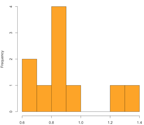
Figure 1. means of ten replicate samples drawn at random from chi-square distribution, df = 1.

Modify the code to draw 100 samples, we get Fig 2.

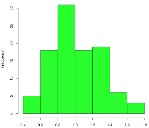
Figure 2. means of 100 replicate samples drawn at random from chi-square distribution, df = 1. Results from Shapiro-Wilks test: W = 0.97426, p-value = 0.04721.

And finally, modify the code to draw one million samples, we get Figure 3.

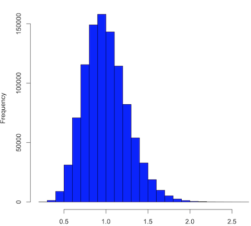
Figure 3. means of one million replicate samples drawn at random from chi-square distribution, df = 1. Normality test will fail to run, sample size of 5000 limit.

How to apply sampling distribution to hypothesis testing

First, a reminder of some definitions.

Estimate = we will always (almost) concern ourselves with how good our sample mean (such values are called estimates) is relative to the population mean, the thing we really want, but can only hope to get an estimate of.

Accuracy = how close to the true value is our measure?

Precision = how repeatable is our measure?

How can we tell if we have a good estimate? We want an estimate with an evaluation for accuracy and for precision. The sampling error provides an assessment of precision, whereas the confidence interval provides a statement of accuracy. We need an estimate of the sampling error for the statistic,

Sample standard error of the mean

We introduced sample error of the mean in section 3.4 of Chapter 3. Everything we measure can have a corresponding statement about how accurate (sampling error) is our estimate! First, we begin by asking, “how accurate is the mean that we estimate from a sample of a population?” How do we answer this? We could prove it in the mathematical sense of proof (and people have and do) OR we can use the computer to help. We’ll try this approach in a minute.

What we will show relates to the standard error of the population mean (SEM) or

, whose equation is shown below.

or equivalently, from the standard deviation we have

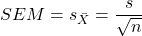
Note that the SEM takes the variance and divides through by the sample size. In general, then, the larger the sample size, the smaller the “error” around the mean. As we work through the different statistical tests, t-tests, analysis of variance, and related, you will notice that the test statistic is calculated as a ratio between a difference or comparison divided by some form of an error measurement. This is to remind you that “everything is variable.”

A note on standard deviation (SD) and standard error of the mean (SEM): SD estimates the variability of a sample of X_i‘s whereas SEM estimates the variability of a sample of means.

Let’s return to our thought problem and see how to demonstrate a solution. First, what is the population? Second, can we get the true population mean?

One way, a direct (but impossible?) approach would be to measure it — get all of the individuals in a population and measure them, then calculate the population mean. Then, we could compare our original sample mean against the true mean and see how close it was. This can be accomplished in some limited cases. For example, the USA conducts a census of her population every ten years, a procedure which costs billions of dollars. We can then compare samples from the different states or counties to the USA mean. And these statistics are indeed available via the census.gov website. But even the census uses sampling — individuals are randomly selected to answer more questions and from this sample trends in the population are inferred.

So, sampling from populations is the way to go for most questions we will encounter. The procedures we will use to show how a sample mean relates to the population mean are general and may be used to show how any estimate of a variable (sample mean and sample standard deviation, etc.), relates to properties of a parameter. We’ll get to the other issues, but for now, think about sample size.

Sampling from populations is necessary and inevitable, and, to a certain extent, under your control. But how many individuals do we need? The quick answer is for me to direct your attention to the equation for the SEM. Can you see in that ratio the secret to obtaining more precise estimates? There are many ways to approach this question, but let’s use the tools from last time, those based on properties of a normal distribution.

If we can view the sampling as having come from a population at least approximately normally distributed for our variable, then we can now examine empirically the effect of different sample sizes on the estimate of the mean.

A hint: variability is important!

From one population we obtain two samples, A and B. Sample sizes are

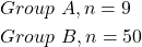
Assume for now that we know the true mean (μ) and standard deviation (σ) for the population. Note. This is one of the points of why we use computer simulation so much to teach statistics — it allows us to specify what the truth is, then see how our statistical tools work or how our assumptions affect our statistically based conclusions.

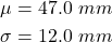
Confidence intervals

Reliability is another word for precision. We define a confidence interval as a statistic to report the reliability of our estimated statistic. We introduced confidence interval in Chapter 3.4. At least in principle, confidence intervals can be calculated for all statistics (mean, variance, etc.,) and for all data types. Confidence intervals define a lower limit, L, and an upper limit, U, and that you are making a statement that you are “95% certain that the true value (parameter value) is between these two limits.

We previously reported how to calculate an approximate confidence intervals for proportions and for NNT; simply multiple standard error estimate by 2. Here we introduce an improved approximate calculation of the 95% confidence interval for the sample mean

where Z is something you would look up from the table of the normal distribution. For a 95% confidence interval, 100% – 95% = 5% and divide 5% by two: the lower limit corresponds to 2.5% and the upper limit corresponds to 2.5% on our normal distribution. We look up the table and we find that Z for 0.025 is 1.96 and that is the value we would plug into our equation above. For large sample sizes, you can get a pretty decent estimate of the confidence interval by replacing 1.96 with “2.”

Questions

1. What is the probability of having a sample mean greater than 50 (mean > 50) for a sample of n = 9 ?

We’ll use a slight modification of the Z-score equation we introduced in Chapter 6.6 — the modification here is that previously we referred to the distribution of Xi‘s and how likely a particular observation would be. Instead, we can use the Z score with the standard normal distribution (aka Z-distribution), approach to solving how likely an estimated sample mean is given the population parameters μ and σ. Recall the Z score

We have everything we need except the SEM, which we can calculate by dividing the standard deviation by squared root of sample size.

For

, σ = 12.0 (given above), and μ = 47, n = 9, plug in the values:

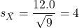
Therefore, after applying the equation for Z score, . This corresponds to how far away from the standard mean of zero.

Look up from the table of normal distribution. The answer is , which corresponds to that is EQUAL to or GREATER than 0.75, which is what we wanted. Translated, this implies that, given the level of variability in the sample, 22.66% of your sample means would be greater than 50! We write: .

Some care needs to be taken when reading these tables — make sure you understand how the direction (less than, greater than) away from the mean is tabulated.

2. Instead of greater, how would you get the probability less than 50?

Total area under the curve is 1 (100%), so subtract .

I recommend that you do these by hand first, then check your answers. You’ll need to be able to do this for exams.

Here’s how to use Rcmdr to do these kind of problems.

Rcmdr: Distributions → Continuous distributions → Normal distribution → Normal probabilities …

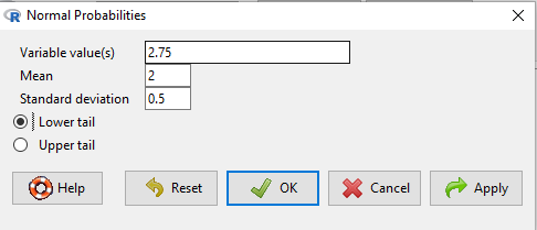
Figure 5. Screenshot Rcmdr menu to get normal probability.

Here’s the answer from Rcmdr

pnorm(c(50), mean=47, sd=12, lower.tail=TRUE)

[1] 0.5987063

3. Now, try a larger sample size. For , what is the probability of having a sample mean greater than 50 ()?

, μ = 47, σ = 12, n = 50 and

Therefore, after applying the equation for Z score, . Look up (Normal table, subtract answer from 1) and we get .

Or 3.84% of your sample means would be greater than 50! We write: .

Said another way: If you have a sample size of 50 () and you obtain a mean greater than 50 then there is only a 3.84% chance that the TRUE MEAN IS 47.

4. What happens if the variability is smaller? Chance σ from 12 to 6 then repeat questions 1 and 4.

5. Repeat the demonstration of Central Limit Theorem and Law of Large Numbers for discrete  distributions

1. binomial distribution. Replace rchisq() with rbinom(n, size, prob) in the replicate() function example. See Chapter 6.5
2. poisson distribution. Replace rchisq() with rpois(n, lambda) in the replicate() function example. See Chapter 6.5

Quiz Chapter 8.3

Sampling distribution and hypothesis testing

Start Quiz

Question

✕

✓

Your answer:

Correct answer:

Next

Please wait..

↺

You got {{SCORE_CORRECT}} out of {{SCORE_TOTAL}}

Your Answers

Chapter 8 contents

• Introduction
• The null and alternative hypotheses
• The controversy over proper hypothesis testing
• Sampling distribution and hypothesis testing
• Tails of a test
• One sample t-test
• Confidence limits for the estimate of population mean
• References and suggested readings

6.4 – Types of probability

Introduction

By probability, we mean a number that quantifies the uncertainty associated with a particular event or outcome. If an outcome is certain to occur, the probability is equal to 1; if an outcome cannot happen, the probability is equal to zero. Most events we talk about in biology have probability somewhere in between.

A basic understanding, or at least an appreciation for probability is important to your education in biostatistics. Simply put, there is no certainty in biology beyond simple expectations like Benjamin Franklin’s famous quip about “death and taxes…”

Discrete probability

You are probably already familiar with discrete probability. For example, what is the probability that a single toss of a fair coin will result in a “heads?” The outcomes of the coin toss are discrete, categorical, either “heads” or “tails.”

And for ten tosses of the coin? And more cogently, what is the probability that you will toss a coin ten times and get all ten “heads?” While different in tone, these are discrete outcomes. An important concept is independence. Are the multiple events independent? In other words, does the toss of coin on the first attempt affect the toss of the coin on the second attempt and so on up to the tenth toss? At least in principle the repeated tosses are independent so to find the probability you just multiply each event’s probability to get the total.

In contrast, if one or more events are not independent but somehow influence the behavior of the next event, then you add the probabilities for each dependent event. We can do better than simply multiply or add events one at a time; depending on the number of discrete outcomes it is very likely that someone has already calculated all possible outcomes and come up with an equation. In the case of the tossing of two coins this is a binomial equation problem and repeat tosses can be modeled by use of the Bernoulli distribution.

Now, try this on for size. What is the probability that the next child born at Kapiolani Medical Center in Honolulu will be assigned female?

We just described a discrete random variable, which can only take on discrete or “countable” numbers.  This distribution of values is the probability mass function. The probability of a one fatal airline accident in a year exactly on 20.1 is practically zero (the area under a point along the curve is zero), so we can get the probability of a range of values around the point as our answer.

Continuous probability

Many events in biology are of degree, not kind. It is kind of awkward to think about it, but for a sample of adult house mice drawn from a population, what is the probability of obtaining a mouse that is 20.0000 grams (g) in weight? Each possible value of body mass for a mouse is considered an event, just like in our example of tossing a coin. But clearly, we don’t expect to get a lot of mice that are exactly 20.0000 g in weight. For variables like body mass, the type of data we collect is continuous, and the probability values need to be rethought along a continuum of possible values and, in turn, how likely each value is for a mouse. Although it is theoretically possible that a mouse could weigh ten pounds, we know by experience that this is impossible. Adult mice weigh between 15 and 50 g or there about.

We just described a continuous random variable, which can take on any value between a specific interval of values. This distribution of values is the probability density function (PDF). The probability of a mouse’s weight falling exactly on 20.1 is practically zero (the area under a point along the curve is zero), so we can get the probability of a range of values around the point as our answer.

In statistical inference, following our measurements of the variables from our sample drawn from a population, we make conclusions with the following kind of caveat: “the mean body mass for this strain of mouse is 20 g.” That is our best estimate of the mean (middle) for the population of mice, more specifically, for the body mass of the mice. Here, the variable body mass is more formally termed a random variable. This implies that there is in fact a true population mean body mass for the mice and that any deviations from that mean are due to chance.

In statistics we don’t settle for a single point estimate of the population mean. You will find most reporting of estimates of random variables is accompanies by a statement like, the mean was 20g with a 95% probability that the true population mean is between 18.9 and 21 g. This is called the 95% confidence interval for the mean and it takes into account how good of an estimate our sample is likely to be relative to the true population value. Not only are we saying that we think the population mean is 20g, but we’re willing to say that we are 95% certain that the true value must be between a lower limit (18.9 g) and and upper limit (21 g). In order to make this kind of statement we have to assume a distribution that will describe the probability of mouse weights. For many reasons we usually assume a normal distribution. Once we make this assumption we can calculate how probable a particular weight is for a mouse.

We introduced how to calculate Confidence Intervals in Chapter 3.4 and will extend this in any chapter that introduces an estimation.

Types of probability

To begin refining our concept of probability, it is sometimes useful to distinguish among kinds of probabilities:

• between theoretical and empirical;
• between subjective and objective.

In most cases, including your statistics book, we would begin our discussion of probability by talking of some probabilities for events we’re familiar with.

1. The theoretical probability of heads appearing the next time you flip a fair coin is 1/2 or 50%. As long as we’re talking about a fair coin, the probability of a heads appearing each time you flip the coin remains 50%. We can check this by conducting and experiment: out of 10 tosses, how many heads appear? The answer would be an empirical probability, and we understand the chance in an objective manner (no interpretation needed).
2. The theoretical probability that a “5” will appear on the face of a fair dice after a toss is 1/6 or 16.667%. Again, as long as we’re talking about a fair dice, the probability of a “5” appearing each time you roll the dice remains 16.667%.
3. The probability that at birth, a human baby’s sex will be male about 1/2 or 50%. This is an empirical probability based on millions of observations. Changes in technology, and ethical standards notwithstanding, the probability will remain the same.
4. The probability of the birth of a Downs syndrome baby is 1/800, but increases with age until by age 45, the chance is 1/12. Again, these are empirical and objective.
5. The probability of winning the Publisher’s Clearing House Sweepstakes is about 1 in 100 million. This probability is theoretical, it is also objective; however, by adding lots of twists to the game, by having multiple opportunities and by giving the appearance that a person must purchase a magazine, some players perceive their chances as increasing or decreasing by their efforts (=subjective).

R and distributions

R offers access to many named distributions. R generally provides four functions available for each.

density (d):the probability density function (PDF) for continuous distributions or the probability mass function (PMF) for discrete distributions.

probability (p): the cumulative distribution function (CDF), which is the chance (probability) of a random variable being less than or equal to a given value

quantile (q): the quantile function (inverse CDF), which returns the value at a given probability

r: draw random numbers from the specified distribution.

Examples of functions for the normal distribution then, are: dnorm(), pnorm(), qnorm(), and rnorm().

Coding example: Find the PDF for x = 0 in a standard normal distribution. # Find the PDF value for x = 0 in a standard normal distribution (mean=0, sd=1)

dnorm(x = 0, mean = 0, sd = 1)

R output

0.398942280401433

Thus, we conclude the chance that x = 0 is about 40%.

Coding example: Find the probability that for x is equal to -1.2 or less in a standard normal distribution.

pnorm(q = -1.2, mean = 0, sd = 1, lower.tail = TRUE)

R output

0.115069670221708

Thus, we conclude the chance that x is equal to or less than -1.2 is about 11.5%.

Coding example: Assuming normal distribution of test scores, what score will 50% of students score? Find the probability that for x is equal to -1.2 or less in a standard normal distribution.

qnorm(0.5, mean = 75, sd = 10)

R output

75

As expected, at 50% it returns the mean. Now, confirm that the lower 25% and upper 75% are 68.26 and 81.75, respectively.

Last coding example, draw random sample of three scores from the same exam.

rnorm(3, mean = 75, sd = 10)

R output

1. 66.0384856946112

2. 69.1887923903669

3. 77.6342297053815

R Commander: Distributions menus give four options

• Quantiles
• Probabilities
• Plot
• Sampling

Questions

1. Define and distinguish, with examples

1. discrete and continuous probability
2. theoretical and empirical probability
3. subjective and objective probability

Quiz Chapter 6.4

Types of probability

Start Quiz

Question

✕

✓

Your answer:

Correct answer:

Next

Please wait..

↺

You got {{SCORE_CORRECT}} out of {{SCORE_TOTAL}}

Your Answers

Chapter 6 contents

• Introduction
• Some preliminaries
• Ratios and proportions
• Combinations and permutations
• Types of probability
• Discrete probability distributions
• Continuous distributions
• Normal distribution and the normal deviate
• Moments
• Chi-square distribution
• t distribution
• F distribution
• References and suggested readings