8.5 – One sample t-test
Introduction.
We’re now talking about the traditional, classical two group comparison involving continuous data types. Thus begins your introduction to parametric statistics. One sample tests involve questions like, how many — what proportion of — people would we expect are shorter or taller than two standard deviations from the mean? This type of question assumes a population and we use properties of the normal distribution and, hence, these are called parametric tests because the assumption is that the data has been sampled from a particular probability distribution.
However, when we start asking questions about a sample statistic (eg, the sample mean), we cannot use the normal distribution directly, ie, we cannot use Z and the normal table as we did before (Chapter 6.7). This is because we do not know the population standard deviation and therefore must use an estimate of the variation (s) to calculate the standard error of the mean.
With the introduction of the t-statistic, we’re now into full inferential statistics-mode. What we do have are estimates of these parameters. The t-test — aka Student’s t-test — was developed for the purpose of testing sample means when the true population parameters are not known.
Note 1: It’s called Student’s t-test after the pseudonym used by William Gosset.
The equation of the one sample t-test. Note the resemblance in form with the Z-score!

where  is the sample standard error of the sample mean (SEM).
For example, weight change of mice given a hormone (leptin) or placebo. The  , but under the null hypothesis, the mean change is “really” zero (
 ). How unlikely is our value of 5 g?
Note 2: Did you catch how I snuck in “placebo” and mice? Do you think the concept of placebo is appropriate for research with mice, or should we simply refer to it as a control treatment? See Ch5.4 – Clinical trials for review.
Speaking of null hypotheses, can you say (or write) the null and alternative hypotheses in this example? How about in symbolic form?
We want to know if our sample mean could have been obtained by chance alone from a population where the true change in weight was zero.
and
and we take these values and plug them into our equation of the t-test
Then recall that Degrees of Freedom are DF = n – 1 so we have DF = 20 – 1 = 19 for the one sample t-test. And the Critical Value is found in the appropriate table of critical values for the t distribution (Fig 1)
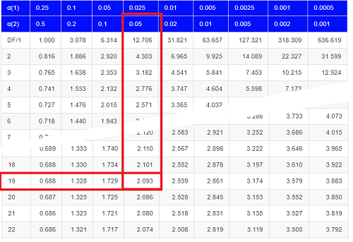
Figure 1. Table of a portion of the Critical values of the t distribution. Red selections highlight critical value for t-test at α = 5% and df = 19.
Note 3: See our table of critical values of t distribution.
Or, and better, use R
qt(c(0.025), df=19, lower.tail=FALSE)
where qt() is function call to find t-score of the pth percentile (cf 3.3 – Measures of dispersion) of the Student t distribution. For a two tailed test, we recall that 0.025 is lower tail and 0.025 is upper tail.
In this example we would be willing to reject the Null Hypothesis if there was a positive OR a negative change in weight.
This was an example of a “two-tailed test” which is “2-tail” or α(2) in Table of critical values of the t distribution.
Critical Value for α(2) = 0.05, df = 19, = 2.093
Do we accept or reject the Null Hypothesis?
A typical inference workflow.
Note the general form of how the statistical test is processed, a form which actually applies to any statistical inference test.
- Identify the type of data
- State the null hypothesis (2 tailed? 1 tailed?)
- Select the test statistic (t-test) and determine its properties
- Calculate the test statistic (the value of the result of the t-test)
- Find degrees of freedom
- For the DF, get the critical value
- Compare critical value to test statistic
- Do we accept or reject the null hypothesis?
And then we ask, given the results of the test of inference, What is the biological interpretation? Statistical significance is not necessarily evidence of biological importance. In addition to statistical significance, the magnitude of the difference — the effect size — is important as part of interpreting results from an experiment. Statistical significance is at least in part because of sample size — the large the sample size, the smaller the standard error of the mean, therefore even small differences may be statistically significant, yet biologically unimportant. Effect size is discussed in Ch9.1 – Chi-square test: Goodness of fit, Ch11.4 – Two sample effect size and Ch12.5 – Effect size for ANOVA.
R Code.
Let’s try a one-sample t-test. Consider the following data set: body mass of four geckos and four Anoles lizards (Dohm unpublished data).
For starters, let’s say that you have reason to believe that the true mean for all small lizards is 5 grams (g).
Geckos: 3.186, 2.427, 4.031, 1.995
Anoles: 5.515, 5.659, 6.739, 3.184
Get the data into R (Rcmdr)
By now you should be able to load this data in one of several ways. If you haven’t already entered the data, check out Part 07. Working with your own data in Mike’s Workbook for Biostatistics.
Once we have our data.frame, proceed to carry out the statistical test.
To get the one-sample t-test in Rcmdr, click on Statistics → Means → Single-sample t-test… Because there is only one numerical variable, Body.mass, that is the only one that shows up in the Variable (pick one) window (Fig 2).
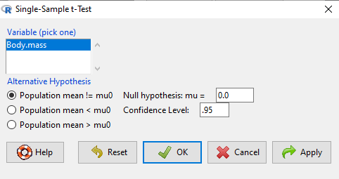
Figure 2. Screenshot Rcmdr single-sample t-test menu.
Type in the value 5.0 in the Null hypothesis: m = u box.
Question 1: Quick! Can you write, in plain old English, the statistical null hypothesis???
Answer 1: For example: No difference between gecko and Anolis lizard mean body mass.
Click OK
The results go to the Output Window.
t.test(lizards$Body.mass, alternative='two.sided', mu=5.0, conf.level=.95)
One Sample t-test
data: lizards$Body.mass
t = -1.5079, df = 7, p-value = 0.1753
alternative hypothesis: true mean is not equal to 5
95 percent confidence interval:
2.668108 5.515892
sample estimates:
mean of x 4.092
end of R output
Let’s identify the parts of the R output from the one sample t-test. R reports the name of the test and identifies
- The
dataset$variableused (lizards$Body.mass). The data set was called “lizards” and the variable was “Body.mass”. R uses the dollar sign ($) to denote the dataset and variable within the data set. - The value of the t test statistic was (t = -1.5079). It is negative because the sample mean was less than the population mean — you should be able to verify this!
- The degrees of freedom, df = 7
- The p-value = 0.1753
- 95% confidence interval of the population mean; lower limit = 2.668108, upper limit = 5.515892
- The sample mean = 4.092
Take a step back and review.
Let’s make sure we “get” the logic of the hypothesis testing we have just completed.
Consider the one-sample t-test.
Step 1. Define HO and HA. The null hypothesis might be that a sample mean,  , is equal to μ = 5.
The alternate is that the sample mean is not equal to 20.
Where did the value 5 come from? It could be a value from the literature (does the new sample differ from values obtained in another lab?). The point is that the value is known in advance, before the experiment is conducted, and that makes it a one-sample t-test.
One tailed hypothesis or two?
We introduced you to the idea of “tails of a test” (Ch08.4). As you should recall, a null/alternative hypothesis for a two-tailed test may be written as
Null hypothesis

versus the alternative hypothesis

where is the sample mean and  is the population mean.
Alternatively, we can write one-tailed tests of null/alternative hypothesis

for the null hypothesis versus the alternative hypothesis

Question 2: Are all possible outcomes of the one-tailed test covered by these two hypotheses?
Answer 2: Yes
Question 3: What was the SEM for this problem?
Answer 3: It would be the sample standard deviation divided by the square root of the sample size.
Step 2. Decide how certain you wish to be (with what probability) that the sample mean is different from μ. As stated previously, in biology, we say that we are willing to be incorrect 5% of the time (Cowles and Davis 1982; Cohen 1994). This means we are likely to correctly reject the null hypothesis 100% – 5% = 95% of the time, which is the definition of statistical power. We do this by setting the Type I error to be 5% (alpha, α = 0.05). The Type I error is the chance that we will reject a null hypothesis, but the true condition in the population we sampled was actually “no difference.”
Step 3. Carry out the calculation of the test statistic. In other words, get the value of t from the equation above by hand, or, if using R (yes!) simply identify the test statistic value from the R output after conducting the one sample t test.
Step 4. Evaluate the result of the test. If the value of the test statistic is greater than the critical value for the test, then you conclude that the chance (the P-value) that the result could be from that population is not likely and you therefore reject the null hypothesis.
Question 4: What is the critical value for a one-sample t-test with df = 7?
Answer 4: From R, we get + 2.365 for the two-tailed test. R code was qt(c(.025), df=7, lower.tail=FALSE)
Hint; you need the table or better, use R
Rcmdr: Distributions → Continuous distributions → t distributions → t quantiles
You also need to know three additional things to answer this question.
- You need to know alpha (α), which we have said generally is set at 5%.
- You also need to know the degrees of freedom (DF) for the test. For a one sample t-test, DF = n – 1, where n is the sample size.
- You also must know whether your test is one or two-tailed.
- You then use the t-distribution (the tables of the t-distribution at the back of your book) to obtain the critical value. Note that if you use R, the actual p-value is returned.
Why learn the equations when I can just do this in R?
Rcmdr does this for you as soon as you click OK. Rcmdr returns the value of the test statistic and the p-value. R does not show you the critical value, but instead returns the probability that your test statistic is as large as it is AND the null hypothesis is true. From our one-sample t-test example, the Rcmdr output. The simple answer is that in order to understand the R output properly you need to know where each item of the output for a particual test comes from and how to interpret it. Thus, the best way is to have the equations available and to understand the algorithmic approach to statistical inference.
And, this is as good of time as any to show you how to skip the RCmdr GUI and go straight to R.
First, create your variables. At the R prompt enter the first variable
liz <- c("G","G","G","G","A","A","A","A")
and then create the second variable
bm <- c(3.186,2.427,4.031,1.995,5.515,5.659,6.739,3.184)
Next, create a data frame. Think of a data frame as another word for worksheet.
lizz <- data.frame(liz,bm)
Verify that entries are correct. At the R prompt type “lizz” wthout the quotes and you should see
lizz
 liz bm
1 G 3.186
2 G 2.427
3 G 4.031
4 G 1.995
5 A 5.515
6 A 5.659
7 A 6.739
8 A 3.184
End of R output
Carry out the t-test by typing at the R prompt the following
t.test(lizz$bm, alternative='two.sided', mu=5, conf.level=.95)
And, like the Rcmdr output we have for the one-sample t-test the following R output
One Sample t-test
data: lizards$Body.mass
t = -1.5079, df = 7, p-value = 0.1753 alternative hypothesis: true mean is not equal to 5
95 percent confidence interval:
2.668108 5.515892
sample estimates:
mean of x
4.092
End of R output
which, as you probably guessed, is the same as what we got from RCmdr.
Question 5: From the R output of the one sample t-test, what was the value of the test statistic?
- -1.5079
- 7
- 0.1753
- 2.668108
- 5.515892
- 4.092
Answer 5: -1.5079
Note 4: BI311 students — On an exam you will be given portions of statistical tables and output from R. Thus you should be able to evaluate statistical inference questions by completing the missing information. For example, if I give you a test statistic value, whether the test is one- or two-tailed, degrees of freedom, and the Type I error rate alpha, you should know that you would need to find the critical value from the appropriate statistical table. On the other hand, if I give you R output, you should know that the p-value and whether it is less than the Type I error rate of alpha would be all that you need to answer the question.
Why fall back on statistical tables? Think of this as a basic skill. In statistics and for some statistical tests, Rcmdr and other software may not provide the information needed to decide that your test statistic is large, and a table in a statistics book is the best way to evaluate the test.
For now, double check Rcmdr by looking up the critical value from the t-table.
Check critical value against our test statistic
Df = 8 – 1 = 7
The test is two-tailed, therefore α(2)
α = 0.05 (note that two-tailed critical value is 2.365. T was equal to 1.51 (since t-distribution is symmetrical, we can ignore the negative sign), which is smaller than 2.365 and so we would agree with Rcmdr — we cannot reject the null hypothesis.
Question 6: From the R output of the one sample t-test, what was the P-value?
- -1.5079
- 7
- 0.1753
- 2.668108
- 5.515892
Answer 6: 0.1753
Question 7: We would reject the null hypothesis
- False
- True
Answer 7: False — p-value, 17.5%, is greater than Type I error of 5%.
Questions
Seven questions, with answers, were provided for you within the text in this chapter. Here’s one more, but without answers.
8. Here’s a small data set for you to try your hand at the one-sample t-test and Rcmdr. The dataset contains cell counts, five counts of the numbers of beads in a liquid with an automated cell counter (Scepter, Millipore USA). The true value is 200,000 beads per milliliter fluid; the manufacturer claims that the Scepter is accurate within 15%. Does the data conform to the expectations of the manufacturer? Write a hypothesis then test your hypothesis with the one-sample t-test. Here’s the data.
| scepter |
| 258900 |
| 230300 |
| 107700 |
| 152000 |
| 136400 |
Quiz Chapter 8.5
One sample t-test
Chapter 8 contents
7.4 – Epidemiology: Relative risk and absolute risk, explained
Risk communication.
Epidemiology is the study of patterns of health and illness of populations. An important task in an epidemiology study is to identify risks associated with disease. Epidemiology is a crucial discipline used to inform about possible effective treatment approaches, health policy, and about the etiology of disease.
Please review terms presented in section 7.1 before proceeding. RR and AR are appropriate for cohort-control and cross-sectional studies (see 2.4 and 5.4) where base rates of exposure and unexposed or numbers of affected and non-affected individuals (prevalence) are available. Calculations of relative risk (RR) and relative risk reduction (RRR) are specific to the sampled groups under study whereas absolute risk (AR) and absolute risk reduction (ARR) pertain to the reference population. Relative risks are specific to the study, absolute risks are generalized to the population. Number needed to treat (NNT) is a way to communicate absolute risk reductions.
An example of ARR and RRR risk calculations using natural numbers.
Clinical trials are perhaps the essential research approach (Sibbald and Roland 1998; Sylvester et al 2017); they are often characterized with a binary outcome. Subjects either get better or they do not. There are many ways to represent risk of a particular outcome, but where possible, using natural numbers is generally preferred as a means of communication, particularly to the general public. Consider the following example (pp 34-35, Gigerenzer 2015): What is the benefit of taking a cholesterol-lowering drug, Pravastatin, on the risk of deaths by heart attacks and other causes of mortality? Press releases (eg, Maugh 1995), from the study stated the following:
“… the drug pravastatin reduced … deaths from all causes 22%”
A subsequent report (Skolbekken 1998) presented the following numbers (Table 1).
Table 1. Reduction in total mortality (5 year study) for people who took Pravastatin compared to those who took placebo.
| Deaths per 1000 people with high cholesterol (> 240 mg/dL) |
No deaths | Cumulative incidence |
||
| Treatment | Pravastatin
(n = 3302) |
a= 32 |
b= 3270 |
CIe |
| Placebo
(n = 3293) |
c= 41 |
d= 3252 |
CIu | |
where cumulative incidence refers to the number of new events or cases of disease divided by the total number of individuals in the population at risk.
Do the calculations of risk
The risk reduction (RR), or the number of people who die without treatment (placebo) minus those who die with treatment (Pravastatin), 
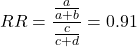
and the cumulative incidence in the exposed (treated) group, CIe, is  , and cumulative incidence in the unexposed (control) group, CIu, is
 . We can calculate another statistic called the risk ratio,
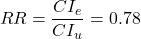
because the risk ratio is less than one, we interpret that statins reduce the risk of mortality from heart attack. In other words, statins lowered the risk by 0.78.
But is this risk reduction meaningful?
Now, consider the absolute risk reduction (ARR) is 
Relative risk reduction, or the absolute risk reduction divided by the proportion of patients who die without treatment, is 
Conclusion: high cholesterol may contribute to increased risk of mortality, but the rate is very low in the population as a whole (the ARR).
Another useful way to communicate benefit is to calculate the Number Needed to Treat (NNT), or the number of people who must receive the treatment to save (benefit) one person. The ideal NNT is a value of one (1), which would be interpreted as everyone improves who receives the treatment. By definition, NNT must be positive; however, a resulting negative NNT would suggest the treatment may cause harm, ie, number needed to harm (NNH).
For this example, the NNT is

therefore, to benefit one person, 111 need to be treated. The flip side of the implications of NNT, although one person may benefit by taking the treatment, 110 ( ) will take the treatment, but will NOT RECEIVE THE BENEFIT, but do potentially get any side effect of the treatment.
Confidence interval for NNT is derived from the Confidence interval for ARR.
For a sample of 100 people drawn at random from a population (which may number in the millions), then repeat the NNT calculation for a different sample of 100 people, do we expect the first and second NNT estimates to be exactly the same number? No, but we do expect them to be close and we can define what we mean by close as we expect each estimate to be within certain limits. While we expect the second calculation to be close to the first estimate, we would be surprised if it was exactly the same. And so, which is the correct estimate, the first or the second? They both are, in the sense that they both estimate the parameter NNT (a property of a population).
We use confidence interval to communicate where we believe the true estimate for NNT to be. Confidence Intervals (CI) allow us to assign a probability to how certain we are about the statistic and whether it is likely to be close to the true value (Altman 1998, Bender 2001). We will calculate the 95% CI for the ARR using the Wald method, then take the inverse of these estimates for our 95% CI. The Wald method assumes normality.
For CI of ARR, we need sample size for control and treatment groups; like all confidence intervals, we need to calculate the standard error of the statistic, in this, case, the standard error (SE) for ARR is approximately

where SE is the standard error for ARR. For our example, we have

The 95% CI for ARR is approximately 
For the Wald estimate, replace the 2 with  , which comes from the normal table for z at

(why the 2 in the equation? Because it is plus or minus so we divide the frequency 0.95 in half) and for our example, we have 
and the inverse for NNT CI is 
Our example exemplifies the limitation of the Wald approach (cf. Altman 1998): our confidence interval includes zero, and doesn’t even include our best estimate of NNT (111).
Note 1: By now I trust you can see differences for results by direct input of the numbers into R and what you get by the natural numbers approach. In part this is because we round in our natural number calculations — remember, while it makes more sense to communicate about whole numbers (people) and not fractions (fractions of people!), rounding through the calculations adds error to the final value. As long as you know the difference and the relevance between approximate and exact solutions, this shouldn’t cause concern.
Software: epiR.
R has many epidemiology packages, epiR and epitools are two. Most of the code presented stems from epiR.
We need to know about our study design in order to tell the functions which statistics are appropriate to estimate. For 2X2 tables, we will use epi.2by2() command, which allows four kinds of studies (Table 2).
Table 2. The method argument in epi.2by2 chooses how to analyze your data based on your study design.
| Method | Description | Notes |
|---|---|---|
| cohort.count | Use this when you follow a set number of people over time and count how many get sick. | This design directly calculates Relative Risk Reduction (RRR) and Absolute Risk Reduction (ARR) because you track baseline risk over time. |
| cohort.time | Use this when you follow people over time and track exactly how long each person was monitored before getting sick. | This calculates rate reductions instead of ARR or RRR because it deals with person-time data rather than raw counts. |
| case.control | Use this when you start with sick people and healthy people and look backwards at their past exposures. | You cannot calculate ARR or RRR here because you do not know the actual baseline risk of the population. |
| cross.sectional | Use this when you take a snapshot of a population at a single point in time to see who is currently exposed and sick. | This calculates prevalence reductions rather than true ARR or RRR because you are not tracking changes over time. |
For our statin example, the design was prospective cohort (ie, cohort.count in epiR package language), not case-control or cross-sectional (review in Chapter 5.4).
library(epiR)
Table1 <- matrix(c(32,3270,41,3252), 2, 2, byrow=TRUE, dimnames = list(c("Statin", "Placebo"), c("Died", "Lived")))
Table1
        Died Lived
Statin    32  3270
Placebo   41  3252
epi.2by2(Table1, method="cohort.count", outcome = "as.columns")
R output
           Outcome + Outcome - Total           Inc risk *
Exposed +         32      3270  3302 0.97  (0.66 to 1.37)
Exposed -         41      3252  3293 1.25  (0.89 to 1.69)
Total             73      6522  6595 1.11  (0.87 to 1.39)

Point estimates and 95% CIs:
-------------------------------------------------------------------
Inc risk ratio                          0.78 (0.49, 1.23)
Inc odds ratio                          0.78 (0.49, 1.24)
Attrib risk in the exposed *           -0.28 (-0.78, 0.23)
Attrib fraction in the exposed (%)    -28.48 (-103.47, 18.88)
Attrib risk in the population *        -0.14 (-0.59, 0.32)
Attrib fraction in the population (%) -12.48 (-37.60, 8.05)
-------------------------------------------------------------------
Uncorrected chi2 test that OR = 1: chi2(1) = 1.147 Pr>chi2 = 0.284
Fisher exact test that OR = 1: Pr>chi2 = 0.292
Wald confidence limits
CI: confidence interval
* Outcomes per 100 population units
The risk ratio we calculated by hand is shown in green in the R output, along with other useful statistics (see ?epi2x2 for help with these additional terms) not defined in our presentation.
We explain results of chi-square goodness of fit (Ch 9.1) and Fisher exact (Ch 9.5) tests in Chapter 9. Suffice to say here, we interpret the p-value (Pr) = 0.284 and 0.292 to indicate that there is no association between mortality from heart attacks with or without the statin (ie, the Odds Ratio, OR, not statistically different from one).
Wait! Where’s NNT and other results?
Use another command in epiR package, epi.tests(), to determine the specificity, sensitivity, and positive (or negative) predictive value.
epi.tests(Table1)
and R returns
          Outcome + Outcome - Total
Test +           32      3270  3302
Test -           41      3252  3293
Total            73      6522  6595

Point estimates and 95% CIs:
--------------------------------------------------------------
Apparent prevalence *                    0.50 (0.49, 0.51)
True prevalence *                        0.01 (0.01, 0.01)
Sensitivity *                            0.44 (0.32, 0.56)
Specificity *                            0.50 (0.49, 0.51)
Positive predictive value *              0.01 (0.01, 0.01)
Negative predictive value *              0.99 (0.98, 0.99)
Positive likelihood ratio                0.87 (0.67, 1.13)
Negative likelihood ratio                1.13 (0.92, 1.38)
False T+ proportion for true D- *        0.50 (0.49, 0.51)
False T- proportion for true D+ *        0.56 (0.44, 0.68)
False T+ proportion for T+ *             0.99 (0.99, 0.99)
False T- proportion for T- *             0.01 (0.01, 0.02)
Correctly classified proportion *        0.50 (0.49, 0.51)
--------------------------------------------------------------
* Exact CIs
Additional statistics are available by saving the output from epi2x2() or epitests() to an object, then using summary(). For example save output from epi.2by2(Table1, method="cohort.count", outcome = "as.columns") to object myEpi, then
summary(myEpi)
look for NNT in the R output
$massoc.detail$NNT.strata.wald
       est    lower    upper
1 -362.377 -128.038  436.481
Thus, the NNT was 362 (compared to 111 we got by hand) with 95% Confidence interval between -436 and +128 (make it positive because it is a treatment improvement).
Note 2: Strata (L. layers), refer to subgroups, for example, sex or age categories (see discussion in Ch05.4). Our examples here are not presented as subgroup analysis, but epiR reports by name strata.
epiR reports a lot of additional statistics in the output and for clarity, I have not defined each one, just the basic terms we need for BI311. As always, see help pages (eg, ?epi.2x2 or ?epitests)for more information about structure of an R command and the output.
We’re good, but we can work the output to make it more useful to us.
Improve output from epiR.
For starters, if we set interpret=TRUE instead of the default, interpret=FALSE, epiR will return a richer response.
fit <- epi.2by2(dat = as.table(Table1), method = "cohort.count", conf.level = 0.95, units = 100, interpret = TRUE, outcome = "as.columns")
fit
R output. In addition to the table of coefficients (above), interpret=TRUE provides more context, shown below
Measures of association strength:
The outcome incidence risk among the exposed was 0.78 (95% CI 0.49 to 1.23) times less than the outcome incidence risk among the unexposed.

The outcome incidence odds among the exposed was 0.78 (95% CI 0.49 to 1.24) times less than the outcome incidence odds among the unexposed.

Measures of effect in the exposed:
Exposure changed the outcome incidence risk in the exposed by -0.28 (95% CI -0.78 to 0.23) per 100 population units. -28.5% of outcomes in the exposed were attributable to exposure (95% CI -103.5% to 18.9%).

Number needed to treat for benefit (NNTB) and harm (NNTH):
The number needed to treat for one subject to be harmed (NNTH) is 362 (NNTH 128 to infinity to NNTB 436).

Measures of effect in the population:
Exposure changed the outcome incidence risk in the population by -0.14 (95% CI -0.59 to 0.32) per 100 population units. -12.5% of outcomes in the population were attributable to exposure (95% CI -37.6% to 8.1%).
That’s quite a bit. Another trick is to get at the table of results. We install a package called broom, which includes a number of ways to handle output from R functions, including those in the epiR package. Broom takes from the TidyVerse environment; tables are stored as tibbles.
Note 3: A tibble (package tibble) is a modified R data frame optimized for the tidyverse that enforces strict data handling and cleaner console printing. Unlike standard data frames, tibbles refuse to automatically simplify into vectors when sliced or guess column names using partial matching. Because of these intentional design choices, tibbles often don’t play well with R functions not written explicitly with the TidyVerse environment in mind.
To convert a data.frame to a tibble,
my_tibble <- as_tibble(my_dataframe)
To convert a tibble back to a standard data.frame
my_dataframe <- as.data.frame(my_tibble)
library(broom)

# Test statistics
tidy(fit, parameters = "stat")
R output
# A tibble: 3 × 4
term statistic df p.value
<chr> <dbl> <dbl> <dbl>
1 chi2.strata.uncor 1.15 1 0.284
2 chi2.strata.yates 0.909 1 0.340
3 chi2.strata.fisher NA NA 0.292
We can convert the tibbles into our familiar data.frame format, and then select only the statistics we want.
# Measures of association
fitD <- as.data.frame(tidy(fit, parameters = "moa")); fitD
R output, all 15 measures of association!
                  term     estimate     conf.low    conf.high
1       RR.strata.wald    0.7783605    0.4914679   1.23272564
2     RR.strata.taylor    0.7783605    0.4914679   1.23272564
3      RR.strata.score    0.8742994    0.6584540   1.10340173
4       OR.strata.wald    0.7761915    0.4876209   1.23553616
5     OR.strata.cfield    0.7761915           NA           NA
6      OR.strata.score    0.7761915    0.4894450   1.23093168
7        OR.strata.mle    0.7762234    0.4718655   1.26668220
8    ARisk.strata.wald   -0.2759557   -0.7810162   0.22910484
9   ARisk.strata.score   -0.2759557   -0.8000574   0.23482532
10     NNT.strata.wald -362.3770579 -128.0383246 436.48140194
11    NNT.strata.score -362.3770579 -124.9910314 425.84844829
12  AFRisk.strata.wald   -0.2847517   -1.0347210   0.18878949
13  PARisk.strata.wald   -0.1381661   -0.5933541   0.31702189
14  PARisk.strata.piri   -0.1381661   -0.3910629   0.11473067
15 PAFRisk.strata.wald   -0.1248227   -0.3760279   0.08052298
We can call out just the statistics we want from this table by calling to the specific elements in the data.frame (rows, columns).
fitD[c(1,4,7,9,12),]
R output
                 term   estimate   conf.low  conf.high
1      RR.strata.wald  0.7783605  0.4914679  1.2327256
4      OR.strata.wald  0.7761915  0.4876209  1.2355362
7       OR.strata.mle  0.7762234  0.4718655  1.2666822
9  ARisk.strata.score -0.2759557 -0.8000574  0.2348253
12 AFRisk.strata.wald -0.2847517 -1.0347210  0.1887895
Software: epitools.
Another useful R package for epidemiology is epitools, but it comes with it’s own idiosyncrasies. We have introduced the standard 2X2 format, with a, b, c, and d cells defined as in Table 1, above. However, epitools does it differently, and we need to update the matrix. By default, epitools has the unexposed group (control) in the first row and the non-outcome (no disease) is in the first column. To match our a,b,c, and d matrix, use the epitools command to change this arrangement with the rev() argument. Now, the analysis will use the contingency table on the right where the exposed group (treatment) is in the first row and the outcome (disease) is in the first column (h/t M. Bounthavong 2021). Once that’s accomplished, epitools returns what you would expect.
Calculate relative risk
risk1 <- 32 / (3270 + 32)
risk2 <- 41 / (3525 + 41)
risk1 - risk2
and R returns
-0.00180638
odds ratio
library(epitools)
oddsratio.wald(Table1, rev = c("both"))
and R returns
$data
              Outcome
Predictor Disease2 Disease1 Total
 Exposed2      517       36   553
 Exposed1      518       11   529
Total         1035       47  1082

$measure
           odds ratio with 95% C.I.
Predictor   estimate      lower      upper
 Exposed2  1.0000000        NA         NA
 Exposed1  0.3049657 0.1535563  0.6056675

$p.value
two-sided
Predictor  midp.exact  fisher.exact    chi.square
Exposed2           NA            NA            NA
Exposed1 0.0002954494  0.0003001641  0.0003517007
odds ratio highlighted in green.
Software: OpenEpi.
R is fully capable of delivering the calculations you need, but sometimes you just want a quick answer. Online, the OpenEpi tools at https://www.openepi.com/ can be used for homework problems. For example, working with count data in 2 X 2 format, select Counts > 2X2 table from the side menu to bring up the data form (Fig 1).
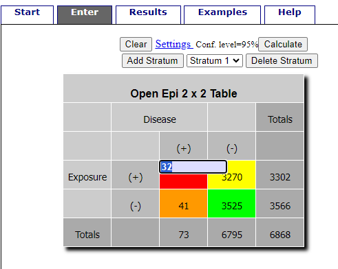
Figure 1. Data entry for 2X2 table at openepi.com.
Once the data are entered, click on the Calculate button to return a suite of results (Fig 2).
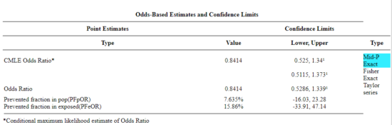
Figure 2. Results for 2X2 table at openepi.com.
Software: RcmdrPlugin.EBM
Note 4: Fall 2023 — I have not been able to run the EBM plugin successfully! The package is still active at CRAN, but looks like it hasn’t been updated since 2015. Simply returns an error message — — on data sets which have in the past performed perfectly. Thus, until further notice, do not use the EBM plugin. Instead, use commands in the epiR package.
This isn’t the place nor can I be the author to discuss what evidence based medicine (EBM) entails (cf. Masic et al. 2008), or what its shortcomings may be (Djulbegovic and Guyatt 2017). Rcmdr has a nice plugin, based on the epiR package, that will calculate ARR, RRR and NNT as well as other statistics. The plugin is called RcmdrPlugin.EBM
install.packages("RcmdrPlugin.EBM", dependencies=TRUE)
After acquiring the package, proceed to install the plug-in. Restart Rcmdr, then select Tools and Rcmdr Plugins (Fig 3).
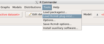
Figure 3. Rcmdr: Tools → Load Rcmdr plugins…
Find the EBM plug-in, then proceed to load the package (Fig 4).
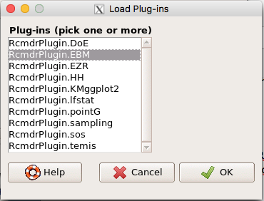
Figure 4. Rcmdr plug-ins available (after first download the files from an R mirror site).
Restart Rcmdr again and the menu “EBM” should be visible in the menu bar. We’re going to enter some data, so choose the Enter two-way table… option in the EBM plug-in (Fig 5)
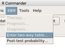
Figure 5. R Commander EBM plug-in, enter 2X2 table menus.
To review, we have the following problem, illustrated with natural numbers and probability tree (Fig 6).
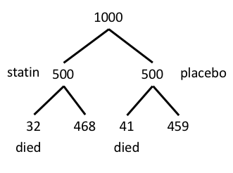
Figure 6. Illustration of probability tree for the statin problem.
Now, let’s enter the data into the EBM plugin. For the data above I entered the counts as
| Lived | Died | |
| Statin | 468 | 32 |
| Placebo | 459 | 41 |
and selected the “Therapy” medical indicator (Fig 7).
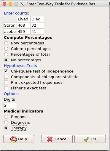
Figure 7. EBM plugin with two-way table completed for the statin problem.
The output from EBM plugin was as follows. I’ve added index numbers in brackets so that we can point to the output that is relevant for our worked example here.
(1) .Table <- matrix(c(468,32,459,41), 2, 2, byrow=TRUE, dimnames = list(c('Drug', 'Placebo'), c('Lived', 'Dead')))
(2) fncEBMCrossTab(.table=.Table, .x='', .y='', .ylab='', .xlab='', .percents='none', .chisq='1', .expected='0', .chisqComp='0', .fisher='0', .indicators='th', .decimals=2)
R output begins by repeating the commands used, here marked by lines (1) and (2). The statistics we want follow in the next several lines of output.
(3) Pearson's Chi-squared test data: .Table X-squared = 1.197, df = 1, p-value = 0.2739
(4) # Notations for calculations Event + Event -Treatment "a" "b" Control "c" "d"
(5)# Absolute risk reduction (ARR) = -1.8 (95% CI -5.02 - 1.42) %. Computed using formula: [c / (c + d)] - [a / (a + b)]
(6)# Relative risk = 1.02 (95% CI 0.98 - 1.06) %. Computed using formula: [c / (c + d)] / [a / (a + b)]
(7)# Odds ratio = 1.31 (95% CI 0.81 - 2.11). Computed using formula: (a / b) / (c / d)
(8) # Number needed to treat = -55.56 (95% CI 70.29 - Inf). Computed using formula: 1 / ARR
9)# Relative risk reduction = -1.96 (95% CI -5.57 - 1.53) %. Computed using formula: { [c / (c + d)] - [a / (a + b)] } / [c / (c + d)]
(10)# To find more about the results, and about how confidence intervals were computed, type ?epi.2by2 . The confidence limits for NNT were computed as 1/ARR confidence limits. The confidence limits for RRR were computed as 1 - RR confidence limits.
end R output
In summary, we found no difference between statin and placebo (P-value = 0.2739) and ARR of -1.8%
Questions.
Data from a case-control study on alcohol use and esophageal cancer (Tuyns et al (1977), example from Gerstman 2014). Cases were men diagnosed with esophageal cancer from a region in France. Controls were selected at random from electoral lists from the same geographical region.
| Esophageal cancer | |||
|
Alcohol grams/day |
Cases | Noncases |
Total |
| > 80 | 96 | 109 |
205 |
|
< 80 |
104 |
666 |
770 |
| Total | 200 | 775 | 975 |
- What was the null hypothesis? Be able to write the hypothesis in symbolic form and as a single sentence.
- What was the alternative hypothesis? Be able to write the hypothesis in symbolic form and as a single sentence.
- What was the observed frequency of subjects with esophageal cancer in this study? And the observed frequency of subjects without esophageal cancer?
- Estimate Relative Risk, Absolute Risk, NNT, and Odds ratio?
- Which is more appropriate, RR or OR? Justify your decision.
- The American College of Obstetricians and Gynecologists recommends that women with an average risk of breast cancer (BC) over 40 get an annual mammogram. Nationally, the sensitivity of mammography is about 68% and specificity of mammography is about 75%. Moreover, mammography involves exposure of women to radiation, which is known to cause mutations. Given that the prevalence of BC in women between 40 and 49 is about 0.1%, please evaluate the value of this recommendation by completing your analysis.
A) In this age group, how many women are expected to develop BC?
B) How many False negative would we expect?
C) How many positive mammograms are likely to be true positives? - “Less than 5% of women with screen-detectable cancers have their lives saved,” (quote from BMC Med Inform Decis Mak. 2009 Apr 2;9:18. doi: 10.1186/1472-6947-9-18): Using the information from question 5, What is the Number Needed to Treat for mammography screening?
Quiz Chapter 7.4
Epidemiology: Relative risk and absolute risk, explained
Chapter 7 contents
- Probability, Risk Analysis
- Epidemiology definitions
- Epidemiology basics
- Conditional Probability and Evidence Based Medicine
- Epidemiology: Relative risk and absolute risk, explained
- Odds ratio
- Confidence intervals
- References and suggested readings
7.3 – Conditional Probability and Evidence Based Medicine
- Conditional probability and risk communication
- Probability and independent events
- Example of multiple, independent events
- Probabilistic risk analysis
- Conditional probability of non-independent events
- Diagnosis from testing
- Standard million
- Per capita rate
- Practice and introduce PPV and test decision criteria
- Evidence Based Medicine
- Software
- Example
- Questions
- Quiz
- Chapter 7 contents
Conditional probability and risk communication.
Conditional probabilities can be used to accurately and effectively convey the risk of specific health outcomes to patients and the public. Tools introduced in this chapter help move from an initial assessment of disease risk to a revised probability after a test result is returned. Although there are other interpretations, here we frame EBM — evidence-based-medicine — as a form of Bayesian decision-making.
This sub-chapter covers a lot of ground. We begin by addressing how probability of multiple events are calculated assuming each event is independent. The assumption of independence is then relaxed, and how to determine probability of an event happening given another event has already occurred, conditional probability, is introduced. Use of conditional probability to interpret results of a clinical test are also introduced, along with the concept of EBM. We also introduce Bayes’ rule and Bayesian probability.
Probability and independent events.
Probability distributions are mathematical descriptions of the probabilities of how often different possible outcomes occur. We also introduced basic concepts related to working with the probabilities involving more than one event.
For review, for independent events, you multiply the individual chance that each event occurs to get the overall probability.
Example of multiple, independent events.
Figure 1. Now that’s a box full of kittens. Creative Commons License, source: https://www.flickr.com/photos/83014408@N00/160490011.
What is the chance of five kittens in a litter of five to be of the same sex? In feral cat colonies, siblings in a litter share the same mother, but not necessarily the same father, superfecundation. Singleton births are independent events, thus the probability of the first kitten is female is 50%; the second kitten is female, also 50%; and so on. We can multiply the independent probabilities (hence, the multiplicative rule), to get our answer:
kittens <- c(0.5, 0.5, 0.5, 0.5, 0.5)
prod(kittens)
[1] 0.03125
Probabilistic risk analysis.
Risk analysis is the use of information to identify hazards and to estimate the risk. A more serious example. Consider the 1986 Space Shuttle Challenger Disaster (Hastings 2003). Among the crew killed was Ellison Onizuka, the first Asian American to fly in space (Fig 2, first on left back row). Onizuka was born and raised on Hawai`i and graduated from Konawaena High School in 1964.

Figure 2. STS-51-L crew: (front row) Michael J. Smith, Dick Scobee, Ronald McNair; (back row) Ellison Onizuka, Christa McAuliffe, Gregory Jarvis, Judith Resnik. Image by NASA – NASA Human Space Flight Gallery, Public Domain.
The shuttle was destroyed just 73 seconds after lift off (Fig 3).

Figure 3. Space Shuttle Challenger launches from launchpad 39B Kennedy Space Center, FL, at the start of STS-51-L. Hundreds of shorebirds in flight. Image by NASA – NASA Human Space Flight Gallery, Public Domain.
This next section relies on material and analysis presented in the Rogers Commission Report June 1986. NASA had estimated that the probability of one engine failure would be 1 in 100 or 0.01; two engine failures would mean the shuttle would be lost. Thus, the probability of two rockets failing at the same time was calculated as 0.01 X 0.01, which is 0.0001 or 0.01%.
NASA had planned to fly the fleet of shuttles 100 times per year, which would translate to a shuttle failure once in 100 years. The Challenger launch on January 28, 1986, represented only the 25th flight of the shuttle fleet.
One difference on launch day was that the air temperature at Cape Canaveral was quite low for that time of year, as low as 22 °F overnight.
Attention was pointed at the large O-rings in the boosters (engines). In all, there were six of these O-rings. Testing suggested that, at the colder air temperatures, the chance that one of the rings would fail was 0.023. Thus, the chance of success was only 0.977. Assuming independence, what is the chance that the shuttle would experience O-ring failure?
shuttle <- c(0.977, 0.977, 0.977, 0.977, 0.977, 0.977)
#probability of success then was
prod(shuttle)
[1] 0.869

#and therefore probability of failure was
1 - prod(shuttle)
[1] 0.1303042
Conditional probability of non-independent events.
But in many other cases, independence of events cannot be assumed. The probability of an event given that another event has occurred is referred to as conditional probability. Conditional probability is used extensively to convey risk. We’ve touched on some of these examples already:
- the risk of subsequent coronary events given high cholesterol;
- the risk of lung cancer given a person smokes tobacco;
- the risk of mortality from breast cancer given that regular mammography screening was conducted.
There are many, many examples in medicine, insurance, you name it. It is even an important concept that judges and lawyers need to be able to handle (eg, discussion in Berry 2008).
A trigger warning: what follows is emotional, traumatic material, provided to emphasize the importance of these concepts, and the far-reaching implications understanding conditional probability can have for us.
A now famous example of conditional probability in the legal arena came from arguments over the chance that a husband or partner who beats his wife will subsequently murder her — this was an argument raised by the prosecution during pre-trial in the 1995 O.J. Simpson trial (The People of the State of California v. Orenthal James Simpson), and successfully argued by O.J. Simpson’s attorneys… judge ruled in favor of the defense and evidence of O.J. Simpson’s prior abuse were not included in trial. Gigerenzer (2002, following discussions by others, eg, Good 1995) and others (eg, Skorupski and Wainer 2015), have called this the Defendent’s Fallacy, the reverse of the Prosecutor’s Fallacy, where the more typical scenario is that the prosecution provides a list of probabilities about characteristics of the defendant, leaving the jury to conclude that no one else could have possibly fit the description ( and 1987).
In the O.J. Simpson case, the argument went something like this. From the CDC we find that the chance of an average woman being murdered by a stranger or an unrelated party was about 1 in 20,000. CDC statistics indicate 1.3 million women are abused each year by their partner or former partner; each year about 1000 women are murdered. One thousand divided by 1.3 million is a small number, so even when there is abuse the argument goes, 99% of the time there is not murder. The Simpson judge ruled in favor of the defense and much of the evidence of prior abuse was excluded.
Something is missing from the defense’s argument. Nicole Brown Simpson did not belong to a population of battered women — she belonged to the population of murdered women. When we ask, if a woman is murdered, what is the chance that she knew her murderer, we find that more than 55% knew their murderer — and of that 55%, 93% were killed by a partner who had a history of prior abuse against the victim.
Instead of looking at all 1.3 million abused women, we isolate a representative cohort of 100,000 abused women to see what mathematically happens to them in a given year:
Group 1: Murdered by their abuser. According to the defense’s rate of 1 in 2,500:
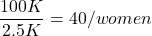
Group 2: Murdered by someone else:
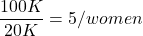
Given that an abused woman was murdered, what is the probability it was done by her abuser?

or 89%.
This is a huge difference from how the Defense portrayed the chance, where they wanted the judge to assume every single one of those 2500 abusers is equally likely to have committed the crime. In reality, we must condition the match on all other available evidence.
The key — Nicole Simpson (and Ron Goldman) were murdered; O.J. Simpson was an ex-partner who had been guilty of assault against Nicole Simpson. Now, it goes from an impossibly small chance, to a much greater chance. Conditional probability, and specifically Bayes’ rule, is used for these kinds of problems. The defense successfully masked a probability that was heavily stacked against their client.
Bayes’ rule provides guidance for how to update the probability of an event based on new evidence. Named after Thomas Bayes (1701- 1761), more generally, Bayes’ rule, described below, is used to quantify conditional probability. Bayesian probability, where probability is interpreted as reasonably expectation instead of frequency of some event. We discuss Bayesian and Frequentist approaches to hypothesis testing in Chapter 8.2.
Note 1: Following our epidemilogy definitions, women murdered by their abuser (Group 2), epidemiology terms, that would be  , the exposure rate in controls, whereas abused woman murdered by her abuser (Group 1), that would be
 , the exposure rate in cases.
Diagnosis from testing.
Let’s turn our attention to medicine. A growing practice in medicine is to claim that decision making in medicine should be based on approaches that give us the best decisions. A search of PubMed texts for “evidence based medicine” found more than 91,944 (13 October 2021, and increase of thirteen thousand since last I looked (10 October, 2019). Evidence based medicine (EBM) is the “conscientious, explicit, judicious and reasonable use of modern, best evidence in making decisions about the care of individual patients” (Masic et al 2008). By evidence, we may mean results from quantitative, systematic reviews, meta-analysis, of research on a topic of medical interest, eg, Cochrane Reviews.
Note 2: Primary research refers to generating or collecting original data in pursuit of tests of hypotheses. Both systematic reviews and meta-analysis are secondary research or “research on research.” As opposed to a literature review, systematic review make explicit how studies were searched for and included; if enough reasonably similar quantitative data are obtained through this process, the reviewer can combine the data and conduct an analysis to assess whether a treatment is effective (De Vries 2018).
As you know, no diagnostic test is 100% fool-proof. For many reasons, test results come back positive when the person truly does not have the condition — this is a false positive result. Correctly identifying individuals who do not have the condition, 100% – false positive rate, is called the specificity of a test.
Think of specificity in this way — provide the test 100 true negative samples (eg, 100 samples from people who do not have cancer) — how many times out of 100 does the test correctly return a “negative”? If 99 times out of 100, then the specificity rate for this test is 99%. Which is pretty good. But the test results mean more if the condition/disease is common; for rare conditions, even 99% is not good enough. Incorrect assignments are rare, we believe, in part because the tests are generally quite accurate. However, what we don’t consider is that detection and diagnosis from tests also depend on the base rate — how frequent the incidence of the condition is in the population. Paradoxically, the lower the base rate, the poorer diagnostic value even a sensitive test may have.
Note 3: This concept, that the base rate effects clinical relevance of interpreting testing — has really important, real-world consequences. It directly bears on clinical testing of cancer and other relatively rare diseases; it also dramatically influences applicability of highly sensitive tests for drug use in clinical samples.
To summarize our jargon for interpreting a test or assay, so far we have
- True positive (a), the person has a disease and the test correctly identifies the person as having the disease.
- False positive (b), test result incorrectly identifies disease; the person does not have the disease, but the test classifies the person as having the disease.
- False negative (c), test result incorrectly classifies person does not have disease, but the person actually has the disease.
- True negative (d), the person does not have the disease and the test correctly categorizes the person as not having the disease.
- Positive predictive value (PPV), the proportion of patients with a positive test result who actually have the disease,
 .
- Negative Predictive Value (NPV), the probability that a person who receives a negative test result really does not have the disease,
 .
- Negative Predictive Value (NPV), the probability that a person who receives a negative test result really does not have the disease,
- Sensitivity of test (Se), the proportion of persons who test positive and do have the disease (true positives):
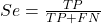
If a test has 75% sensitivity, then out of 100 individuals who do have the disease, then 75 will test positive (TP = true positive). - Specificity of a test (Sp), refers to the rate that a test correctly classifies a person that does not have the disease (TN = true negatives):
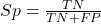
If a test has 90% specificity, then out of 100 individuals who truly do not have the disease, then 90 will test negative (= true negatives).
A worked example. A 50 year old male patient is in the doctor’s office. The doctor is reviewing results from a diagnostic test, eg, a FOBT — fecal occult blood test — a test used as a screening tool for colorectal cancer (CRC). The doctor knows that the test has a sensitivity of about 75% and specificity of about 90%. Prevalence of CRC in this age group is about 0.2% (cf NCI SEER). The prevalence is also the prior probability — the baseline rate of the condition in the population before a test is taken. Figure 4 shows our probability tree using our natural numbers approach (Fig 4).
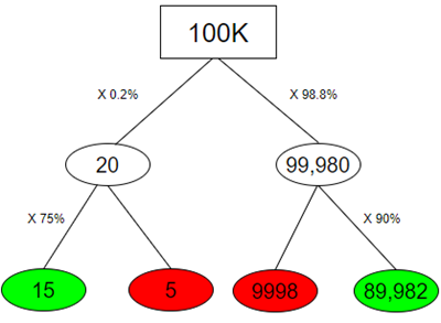
Figure 4. Probability tree for FOBT test; Good test outcomes shown in green: TP stands for true positive and TN stands for true negative. Poor outcomes of a test shown in red: FN stands for false negative and FP stands for false positive.
Note 4: Since U.S. Preventative Task Force (2021), FOBT has largely been replaced by Fecal Immunochemical Test (FIT): sensitivity 74%, specificity 95%, and Multitarget Stool DNA Test: sensitivity 76%, specificity 90%. Cologuard combines both: sensitivity 92%, specificity 97% (cf discussion in Imperiale et al 2014).
- The U.S. Supreme Court (Kennedy v. Braidwood Management, Inc) supported USPSTF’s authority to recommend preventive services covered by insurers (see 2025 article by R. Payerchin in Medical Economics).
The associated probabilities for the four possible outcomes of these kinds of tests (eg, what’s the probability of a person who has tested positive in screening tests actually has the disease?) are shown in Table 1.
Table 1. A 2 X 2 table of possible outcomes of a diagnostic test.
| Person really has the disease | ||
| Test Result | Yes | No |
| Positive | a TP |
b FP |
| Negative | c FN |
d TN |
We want the posterior probability — the chance that a positive test result is a true positive. Bayes’ rule is often given in probabilities,

Bayes’ rule, where truth is represented by either D (the person really does have the disease”) or ND (the person really does not have the disease”) and ⊕ is symbol for “exclusive or” and reads “not D” in this example.
An easier way to see this is to use frequencies and our table instead (Table 1, numbers in Figure 4).
Now, the formula is

Simplified Bayes’ rule, where a is the number of people who test positive and DO HAVE the disease and b is the number of people who test positive and DO NOT have the disease. Thus,  , the posterior probability was

or 0.15%. Because the condition is so rare (0.2% prior) and the test generates a very high number of False Positives (9,998), getting a positive result actually lowers oour confidence slightly from the base rate (from 0.2% down to 0.15%). This occurs because the test is highly unreliable in screening this specific population — it’s known as the base rate fallacy. Thus, the chance that a positive FOBT test for our 50 year old male patient is 99.85% likely wrong.
Standardized million.
Where did the 100,000 come from? We discussed this in chapter 2: it’s a simple trick to adjust rates to the same population size. We use this to work with natural numbers instead of percent or frequencies. You choose to correct to a standardized population based on the raw incidence rate. A rough rule of thumb:
Table 2. Relationship between standard population size and incidence rate.
| Raw IR rate about | IR | Standard population |
| 1/10 | 10% | 1000 |
| 1/100 | 1% | 10,000 |
| 1/1000 | 0.1% | 100,000 |
| 1/10,000 | 0.01% | 1,000,000 |
| 1/100,000 | 0.001% | 10,000,000 |
| 1/1,000,000 | 0.0001% | 100,000,000 |
The raw incident rate is simply the number of new cases divided by the total population.
Per capita rate.
Yet another standard manipulation is to consider the average incidence per person, or per capita rate. The Latin “per capita” translates to “by head” (Google translate), but in economics, epidemiology, and other fields it is used to reflect rates per person. Tuberculosis is a serious infectious disease of primarily the lungs. Incidence rates of tuberculosis in the United States have trended down since the mid 1900s: 52.6 per 100K in 1953 to 2.7 per 100K in 2019 (CDC). Corresponding per capita values are 5.26 x 10⁻⁴ and 2.7 x 10⁻⁵, respectively. Divide the rate by 100,000 to get per person rate.
Practice and introduce PPV and test decision criteria.
Let’s break these problems down, and in doing so, introduce some terminology common to the field of “risk analysis” as it pertains to evaluating assay and diagnotistc tests in biology and epidemiology. Our first example considers the fecal occult blood test, FOBT, test. Blood in the stool may (or may not) indicate polys or colon cancer (Park et al 2010).
A table like the one shown above (Table 1) will appear again and again throughout this and subsequent chapters, but in different forms. We start with Table 3.
Table 3. A 2 X 2 table of possible outcomes of FOBT test.
| Person really has the disease | |||
| Yes | No | ||
| Positive | 15 | 9998 | PPV = 15/(15+9998) = 0.15% |
| Negative | 5 | 89,982 | NPV = 89982/(89982+5) = 99.99% |
We want to know how good is the test, particularly if the goal is early detection? This is conveyed by the PPV, positive predictive value of the test. Unfortunately, the prevalence of a condition is also at play: the lower the prevalence, the lower the PPV must be, because most positive tests will be false when population prevalence is low.
Youden (1950) proposed a now widely adopted index that summarizes how effective a test is. Youden’s J is the sum of specificity and sensitivity minus one.

where Se stands for sensitivity of the test and Sp stands for sensitivity of the test.
Youden’s J takes on values between 0, for a terrible test, and 1, for a perfect test. For our FOBT example, Youden’s J was 0.65. This statistic looks like it’s independent of prevalence, but it’s use as a decision criterion (eg, a cutoff value, above which test is positive, below test is considered negative), assumes that the cost of misclassification (false positives, false negatives) are equal. Prevalence affects number of false positives and false negatives for a given diagnostic test, so any decision criterion based on Youden’s J will also be influenced by prevalence (Smits 2010).
Youden’s J is insensitive to base rates and therefore may be of little practical use in the field. Unsurprisingly, other tools are available, including Matthew’s Correlation Coefficient (MCC),

and the positive and negtive Clinical Utility Index (CUI+, CUI-),

or the F1-score,

epiR will calculate Youden’s J, but the others are either calculated by hand or by way of additional packages. So, we’ll provide a function.
R code to calculate testing decision criteria — code genereated with Gemini AI assistance.
run_screening_wizard <- function() {
# 1. Sequential user prompts starting with cell a
cat("--- 2x2 Matrix Entry Wizard ---\n")
a <- as.numeric(readline(prompt = "Enter cell a (True Positives, TP): "))
b <- as.numeric(readline(prompt = "Enter cell b (False Positives, FP): "))
c <- as.numeric(readline(prompt = "Enter cell c (False Negatives, FN): "))
d <- as.numeric(readline(prompt = "Enter cell d (True Negatives, TN): "))

# 2. Map cells to short variables for calculation
tp <- a
fp <- b
fn <- c
tn <- d

# 3. Construct and print the visual 2x2 matrix
user_matrix <- matrix(
c(tp, fp, fn, tn),
nrow = 2,
byrow = TRUE,
dimnames = list(Test = c("+", "-"), Disease = c("+", "-"))
)
cat("\n[+] Captured Matrix:\n")
print(user_matrix)

# 4. Run background metrics math
sensitivity <- tp / (tp + fn)
specificity <- tn / (tn + fp)
ppv <- tp / (tp + fp)
if (is.nan(ppv)) ppv <- 0

youden_j <- sensitivity + specificity - 1
cui_pos <- sensitivity * ppv

f1_score <- 2 * ((ppv * sensitivity) / (ppv + sensitivity))
if (is.nan(f1_score)) f1_score <- 0

mcc_num <- (tp * tn) - (fp * fn)
mcc_den <- sqrt(as.numeric(tp + fp) * as.numeric(tp + fn) *
as.numeric(tn + fp) * as.numeric(tn + fn))
mcc <- if (mcc_den == 0) 0 else mcc_num / mcc_den

# 5. Compile into the copy/paste ready console matrix
output_matrix <- matrix(
c(round(youden_j, 4), "No", "Good (Overly optimistic baseline)",
round(mcc, 4), "Yes", "Poor (Correctly captures imbalance)",
round(cui_pos, 4), "Yes", "Unacceptable clinical utility",
round(f1_score, 4), "Yes", "Near-total prediction failure"),
nrow = 4, byrow = TRUE
)

dimnames(output_matrix) <- list(
c("Youden's J Index", "MCC", "CUI+", "F1-Score"),
c("Value", "Base_Rate_Dep", "Console_Interpretation")
)

final_df <- as.data.frame(output_matrix)

# 6. Print and invisibly return the dataframe
cat("\n[+] Resulting Metrics Table (Copy/Paste Ready):\n")
print(final_df)
return(invisible(final_df))
}

# Run the function at the R command prompt.
run_screening_wizard()
End R code.
Thus, using a metric sensitive to low base rate, our FOBT tests are (modified from R output)
Table 4. Decision criteria.
| Value | Base rate dependent? | Interpretation | |
 |
0.65 | No | Good |
 |
0.0306 | Yes | Poor |
 |
0.0011 | Yes | Unacceptable clinical utility |
 |
0.0030 | Yes | Near-total prediction failure |
Another worked example. A study on cholesterol-lowering drugs (statins) reported a relative risk reduction of death from cardiac event by 22%. This does not mean that for every 1000 people fitting the population studied, 220 people would be spared from having a heart attack. In the study, the death rate per 1000 people was 32 for the statin versus 41 for the placebo — recall that a placebo is a control treatment offered to overcome potential patient psychological bias (see Chapter 5.4). The absolute risk reduction due to statin is only 41 – 32 or 9 in 1000 or 0.9%. By contrast, relative risk reduction is calculated as the ratio of the absolute risk reduction (9) divided by the proportion of patients who died without treatment (41), which is 22% (LIPID Study Group 1998).
Note that risk reduction is often conveyed as a relative rather than as an absolute number. The distinction is important for understanding arguments based in conditional probability. Thus, the question we want to ask about a test is summarized by absolute risk reduction (ARR) and number needed to treat (NNT), and for problems that include control subjects, relative risk reduction (RRR). We expand on these topics in the next section, 7.4 – Epidemiology: Relative risk and absolute risk, explained.
Evidence Based Medicine.
One culture change in medicine is the explicit intent to make decisions based on evidence (Masic et al 2008). Of course, the joke then is, well, what were doctors doing before, diagnosing without evidence? The comic strip xkcd offers one possible answer (Fig 5).
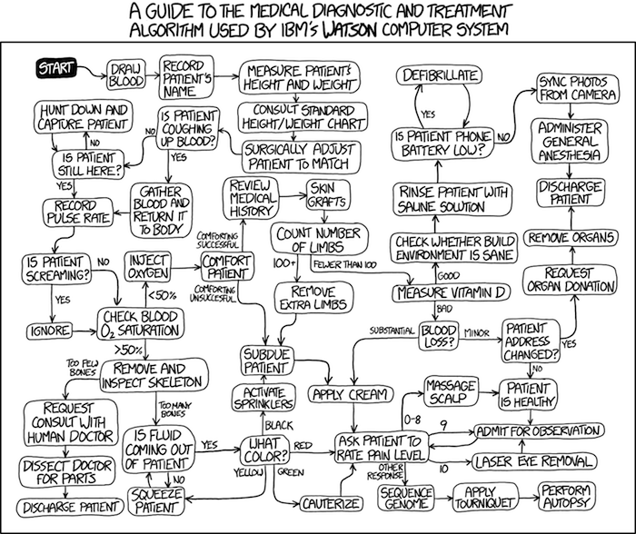
Figure 5. A summary of “evidence based medical” decisions, perhaps? “Watson Medical Algorithm,” https://xkcd.com/1619/.
As you can imagine, there’s considerable reflection about the EBM movement (see discussions in response to Accad and Francis 2018, eg, Goh 2018). More practically, our objective is for you to be able to work your way through word problems involving risk analysis. You can expect to be asked to calculate, or at least set up for calculation, any of the statistics listed above (eg, False negative, false positive, etc.). Practice problems are listed at the end of this section, and additional problems are provided to you (Homework 4). You’ll also want to check your work, and in any real analysis, you’d most likely want to use R.
Software.
R has several epidemiology packages, and with some effort, can save you time. Another option is to run your problems in OpenEpi, a browser-based set of tools. OpenEpi is discussed with examples in the next section, 7.4.
Here, we illustrate some capabilities of the epiR package, expanded more also in the next section, 7.4. We’ll use the example from Table 3.
R code
library(epiR)
Table3 <- matrix(c(15, 5, 9998, 89982), nrow = 2, ncol = 2)
epi.tests(Table3)
R output
         Outcome + Outcome -   Total
Test +          15      9998   10013
Test -           5     89982   89987
Total           20     99980  100000

Point estimates and 95% CIs:
--------------------------------------------------------------
Apparent prevalence *                      0.10 (0.10, 0.10)
True prevalence *                          0.00 (0.00, 0.00)
Sensitivity *                              0.75 (0.51, 0.91)
Specificity *                              0.90 (0.90, 0.90)
Positive predictive value *                0.00 (0.00, 0.00)
Negative predictive value *                1.00 (1.00, 1.00)
Positive likelihood ratio                  7.50 (5.82, 9.67)
Negative likelihood ratio                  0.28 (0.13, 0.59)
False T+ proportion for true D- *          0.10 (0.10, 0.10)
False T- proportion for true D+ *          0.25 (0.09, 0.49)
False T+ proportion for T+ *               1.00 (1.00, 1.00)
False T- proportion for T- *               0.00 (0.00, 0.00)
Correctly classified proportion *          0.90 (0.90, 0.90)
--------------------------------------------------------------
* Exact CIs
Oops! I wanted PPV, which by hand calculation was 0.15%, but R reported “0.00?” This is a significant figure reporting issue. The simplest solution is to submit options(digits=6) before the command, then save the output from epi.tests() to an object and use summary(). For example
options(digits=6)
myEpi <- epi.tests(Table3)
summary(myEpi)
And R returns
     statistic           est        lower        upper
1           ap  0.1001300000 0.0982761568  0.102007072
2           tp  0.0002000000 0.0001221693  0.000308867
3           se  0.7500000000 0.5089541283  0.913428531
4           sp  0.9000000000 0.8981238085  0.901852950
5      diag.ac  0.8999700000 0.8980937508  0.901823014
6      diag.or 27.0000000000 9.8110071871 74.304297826
7         nndx  1.5384615385 1.2265702376  2.456532054
8       youden  0.6500000000 0.4070779368  0.815281481
9       pv.pos  0.0014980525 0.0008386834  0.002469608
10      pv.neg  0.9999444364 0.9998703379  0.999981958
11      lr.pos  7.5000000000 5.8193604069  9.666010707
12      lr.neg  0.2777777778 0.1300251423  0.593427490
13      p.rout  0.8998700000 0.8979929278  0.901723843
14       p.rin  0.1001300000 0.0982761568  0.102007072
15      p.tpdn  0.1000000000 0.0981470498  0.101876192
16      p.tndp  0.2500000000 0.0865714691  0.491045872
17      p.dntp  0.9985019475 0.9975303919  0.999161317
18      p.dptn  0.0000555636 0.0000180416  0.000129662
There we go — pv.pos reported as 0.0014980525, which, after turning to a percent and rounding, we have 0.15%. Note also the additional statistics provided — a good rule of thumb — always try to save the output to an object, then view the object, eg, with summary(). Refer to help pages for additional details of the output (?epi.tests).
What about R Commander menus?
Note 3: Confirmed Fall 2026 — I have not been able to run the EBM plugin successfully! Simply returns an error message — — on data sets which have in the past performed perfectly. Thus, until further notice, do not use the EBM plugin. Instead, use commands in the epiR package. I’m leaving the text here on the chance the error with the plugin is fixed.
Rcmdr has a plugin that will calculate ARR, RRR and NNT. The plugin is called RcmdrPlugin.EBM (Leucuta et al 2014) and it would be downloaded as for any other package via R.
Download the package from your selected R mirror site, then start R Commander.
install.packages("RcmdrPlugin.EBM")
From within R Commander (Fig 6), select
Tools → Load Rcmdr plug-in(s)…
Figure 6. To install an Rcmdr plugin, first go to Rcmdr → Tools → Load Rcmdr plug-in(s)…
Next, select from the list the plug-in you want to load into memory, in this case, RcmdrPlugin.EBM (Fig 7).
Figure 7. Select the Rcmdr plugin, then click the “OK” button to proceed.
Restart Rcmdr again (Fig 8),
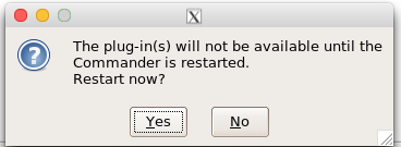
Figure 8. Select “Yes” to restart R Commander and finish installation of the plug-in.
and the menu “EBM” should be visible in the menu bar (Fig 9).
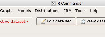
Figure 9. After restart of R Commander the EBM plug-in is now visible in the menu.
Note that you will need to repeat these steps each time you wish to work with a plug-in, unless you modify your .RProfile file. See
Rcmdr → Tools → Save Rcmdr options…
Clicking on the EBM menu item brings up the template for the Evidence Based Medicine module. We’ll mostly work with 2 X 2 tables (eg, see Table 1) , so select the “Enter two-way table…” option to proceed (Fig 10).
Figure 10. Select “Enter two-way table…”.
And finally, Figure 11 shows the two-way table entry cells along with options. We’ll try a problem by hand then use the EBM plugin to confirm and gain additional insight.
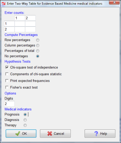
Figure 11. Two-way table Rcmdr EBM plug-in.
For assessing how good a test or assay is, use the Diagnosis option in the EBM plugin. For situations with treated and control groups, use Therapy option. For situations in which you are comparing exposure groups (eg, smokers vs non-smokers), use the Prognosis option.
Example.
Here’s a simple one (problem from Gigerenzer 2002).
About 0.01% of men in Germany with no known risk factors are currently infected with HIV. If a man from this population actually has the disease, there is a 99.9% chance the tests will be positive. If a man from this population is not infected, there is a 99.9% chance that the test will be negative. What is the chance that a man who tests positive actually has the disease?
Start with the reference, or base population (Figure 12). It’s easy to determine the rate of HIV infection in the population if you use numbers. For 10,000 men in this group, exactly one man is likely to have HIV (0.0001X10,000), whereas 9,999 would not be infected.
For the man who has the disease it’s virtually certain that his results will be positive for the virus (because the sensitivity rate = 99.9%). For the other 9,999 men, one will test positive (the false positive rate = 1 – specificity rate = 0.01%).
Thus, for this population of men, for every two who test positive, one has the disease and one does not, so the probability even given a positive test is only 100*1/2 = 50%. This would also be the test’s Positive Predictive Value.
Note that if the base rate changes, then the final answer changes! For example, if the base rate was 10%
It also helps to draw a tree to help you determine the numbers (Fig 12)
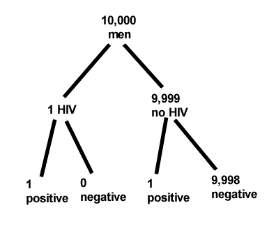
Figure 12. Draw a probability tree to help with the frequencies.
From our probability tree in Figure 12 it is straight-forward to collect the information we need.
- Given this population, how many are expected to have HIV? Two.
- Given the specificity and sensitivity of the assay for HIV, how many persons from this population will test positive? Two.
- For every positive test result, how many men from this population will actually have HIV? One.
Thus, given this population with the known risk associated, the probability that a man testing positive actually has HIV is 50% (=1/(1+1)).
Use the EBM plugin. Select two-way table, then enter the values as shown in Fig 13.
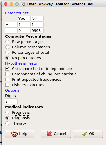
Figure 13. EBM plugin with data entry.
Select the “Diagnosis” option — we are answering the question: How probable is a positive result given information about sensitivity and specificity of a diagnosis test. The results from the EBM functions are given below
Rcmdr> .Table
      Yes No
   +  1    1
   -  0 9998
Rcmdr> fncEBMCrossTab(.table=.Table, .x='', .y='', .ylab='', .xlab='',
Rcmdr+ .percents='none', .chisq='1', .expected='0', .chisqComp='0', .fisher='0',
Rcmdr+ .indicators='dg', .decimals=2)
# Notations for calculations
        Disease + Disease -
Test +      "a"         "b"
Test -      "c"         "d"
# Sensitivity (Se) = 100 (95% CI 2.5 - 100) %. Computed using formula: a / (a + c)
# Specificity (Sp) = 99.99 (95% CI 99.94 - 100) %. Computed using formula: d / (b + d)
# Diagnostic accuracy (% of all correct results) = 99.99 (95% CI 99.94 - 100) %. Computed using formula: (a + d) / (a + b + c + d)
# Youden's index = 1 (95% CI 0.02 - 1). Computed using formula: Se + Sp - 1
# Likelihood ratio of a positive test = 9999 (95% CI 1408.63 - 70976.66). Computed using formula: Se / (Sp - 1)
# Likelihood ratio of a negative test = 0 (95% CI 0 - NaN). Computed using formula: (1 - Se) / Sp
# Positive predictive value = 50 (95% CI 1.26 - 98.74) %. Computed using formula: a / (a + b)
# Negative predictive value = 100 (95% CI 99.96 - 100) %. Computed using formula: d / (c + d)
# Number needed to diagnose = 1 (95% CI 1 - 40.91). Computed using formula: 1 / [Se - (1 - Sp)]
Note that the formulas used to calculate Sensitivity, Specificity, etc., follow our Table 1 (compare to “Notations for calculations”). The use of EBM provides calculations of our confidence intervals.
Questions.
- The sensitivity of the fecal occult blood test (FOBT) is reported to be 0.68. What is the False Negative Rate?
- The specificity of the fecal occult blood test (FOBT) is reported to be 0.98. What is the False Positive Rate?
- For men between 50 and 54 years of age, the rate of colon cancer is 61 per 100,000. If the false negative rate of the fecal occult blood test (FOBT) is 10%, how many persons who have colon cancer will test negative?
- For men between 50 and 54 years of age, the rate of colon cancer is 61 per 100,000. If the false positive rate of the fecal occult blood test (FOBT) is 10%, how many persons who do not have colon cancer will test positive?
- A study was conducted to see if mammograms reduced mortality
Mammogram Deaths/1000 women No 4 Yes 3 data from Table 5-1 p. 60 Gigerenzer (2002)
What is the RRR? - A study was conducted to see if mammograms reduced mortality
Mammogram Deaths/1000 women No 4 Yes 3 data from Table 5-1 p. 60 Gigerenzer (2002)
What is the NNT? - Does supplemental Vitamin C decrease risk of stroke in Type II diabetic women? A study conducted on 1923 women, a total of 57 women had a stroke, 14 in the normal Vitamin C level and 32 in the high Vitamin C level. What is the NNT between normal and high supplemental Vitamin C groups?
- Sensitivity of a test is defined as
A. False Positive Rate
B. True Positive Rate
C. False Negative Rate
D. True Negative Rate - Specificity of a test is defined as
A. False Positive Rate
B. True Positive Rate
C. False Negative Rate
D. True Negative Rate - In thinking about the results of a test of a null hypothesis, Type I error rate is equivalent to
A. False Positive Rate
B. True Positive Rate
C. False Negative Rate
D. True Negative Rate - During the Covid-19 pandemic, number of reported cases each day were published. For example, 155 cases were reported for 9 October 2020 by Department of Health. What is the raw incident rate?
Quiz Chapter 7.3
Conditional Probability and Evidence Based Medicine
Chapter 7 contents
- Introduction
- Epidemiology definitions
- Epidemiology basics
- Conditional Probability and Evidence Based Medicine
- Epidemiology: Relative risk and absolute risk, explained
- Odds ratio
- Confidence intervals
- References and suggested readings
5.4 – Clinical trials
Introduction
Two areas of inquiry have contributed enormously to our understanding of experimental design: agriculture research (Verdooren 2020) and human subject clinical trials. This page outlines types of clinical trial designs and briefly introduces the subject of research ethics with human subject research (Huang and Hadian 2006). After completing this page, the reader will be able to identify key clinical trial types and recognize the fundamental ethical principles governing human subject research.
Although this page does not address the many concerns for ethical research in ecology and environmental studies, many parallels can be drawn (Crozier and Schulte-Hostedde 2014, Samuel and Richie 2022). To name just one example, both disciplines mandate a “do no harm,” principle. In clinical research this amounts to minimizing risks to human subjects; in environmental and ecology studies, acknowledging experimental studies through sampling or chemical releases can damage ecosystems (Resnik 2009).
An outline of clinical trials
Much has been written about biomedical research study design; a couple of accessible articles that can supplement the material presented here include Benson and Hart 2000, Concato et al 2000, Gabriella 2012. Even if you never work in clinical research, understanding how clinical trials are designed and under what circumstances limitations of particular designs arise is helpful to all of us who do experimental work. In Mike’s Workbook for Biostatistics we will present descriptions of research activities and step through situations where you will attempt to align the research by analogy to clinical trials. A second approach to learning about experimental design is to read about someone’s study, and reworking it in terms of a clinical trial design perspective. We will use a discussion of clinical trials, used in biomedical research to investigate effectiveness of treatments of disease, as our starting point for learning how statistics informs experimentation.
Types of clinical trials are distinguished by their design and include:
Case studies are a thorough analysis of an individual patient, or a few individuals (a group), focusing on symptoms, diagnostics, treatments and outcomes. Case studies can utilize quantitative or qualitative research methods. Case studies, of course, are not restricted to medical research. The main disadvantage of case studies is that by definition they are not generalizable to the population and, by their very nature, researcher subjectivity (choice of diagnostics, interpretations) and other kinds of bias may be challenging to control. A 2025 case study received considerable news coverage: a 60 year old man developed bromism — a toxic condition resulting from excessive exposure to bromides — consulting ChatGPT for health information (Eichenberger et al 2025).
Experimental studies are just that, research designs that apply techniques of experimental science — controls, randomization, attempts to account for sources of bias. They are intended to make direct comparisons among subjects assigned by the researcher to treatment groups. By definition experiments are longitudinal studies. Longitudinal studies are experimental or observational studies in which multiple observations are recorded for each individual and individuals are tracked over time. Many excellent resources about experimental design, beginning with R.A. Fisher’s 1935 book, The design of experiments, to Scheiner and Gurevitch (Editors) 2001, Design and Analysis of Ecological Experiments (2nd edition), to the many books on randomized control trials, eg, the 5th edition of Designing clinical research (2022), edited by Browner et al.
Observational (or epidemiological) studies — no direct intervention is administered and so observational studies tend to be retrospective; we identify individuals with and without the condition and attempt to identify associations between the condition and any number of potential causal factors.
Cross-sectional studies are examples of descriptive study designs. They take observations at one point in time on a variety of individuals. It can be used to associate factors with the condition in question, and can be used to estimate the prevalence of a condition in the population. Omair (2015) provides an accessible summary of case and cross-sectional study designs.
Cross-sectional studies are referred to as method = cross.sectional in the package epiR.
Cohort studies involve a group of subjects (eg, patients) who receive the same treatment at the same time. A cohort consists of subjects who are linked in some way. It could be a trivial link, like the cohorting done at university (all incoming Freshmen students who enroll for a class offered at 9:30AM), or it could be based on shared experience due to an exposure event (eg, all passengers on a jet traveling with an index case or “patient zero”).
- Prospective cohort studies enroll people as cohorts at the beginning of a study and follow them over time
- Retrospective cohort studies may utilize archived records.
Cohort and other variations of observational studies (eg, case control, test-negative design), can establish associations between risk factors and conditions or specific adverse events, but cannot by themselves establish cause and effect (Benson and Hartz 2000). A search of PUBMED for “cohort study” reports more than 3.2 million studies since 1914. A 2025 prospective cohort study with more than 1800 pregnant women found no change in risk of major birth defects after maternal mRNA COVID-19 vaccination in the first trimester of pregnancy (Kayser et al 2025).
Cohort studies are referred to as method = cohort.count in the package epiR.
Case control studies are similar to cohort studies, except they are retrospective. Case refers to subjects with one or more characteristics of interest. Used to infer the exposure risk factor by evaluating historical records. Omair (2016) provides an accessible summary of cohort and case control study designs. Designed to identify associations between exposure and particular outcomes, case control studies are retrospective and observational studies: Retrospective because the outcomes are already known, and observational because the event was caused by nature, not experiment. In principle, researchers identify a number of cases with a particular outcome (eg, lung cancer), then attempt to match cases to individuals who do not have the outcome (controls). Work is done to look back to see if the exposure (eg, smoking) is more frequent in the case group than the control group.
Case control studies have several advantageous compared to other approaches: rapid to conduct compared to longitudinal studies (the even has already happened), and efficient because small sample sizes may be enough to reach conclusions. Among their limitations, however, is the problem of how to match cases with controls. Obvious matching accomplished by grouping by age categories, body mass index, gender, socio-economic status, and so on. Three papers authored by Wacholder published in American Journal of Epidemiology 1992 describe in detail, from theory to practice, case control selection (Wacholder 1992abc). A search of PUBMED for “case control” reports more than 400 thousand studies since 1950. A 2025 case control study with more than one million records found no effect of aluminum adjuvant in childhood vaccines on chronic autoimmunity, atopy or allergy, and neurodevelopmental disorders (Andersson et al 2025).
Case control studies are referred to as method = case.control in the package epiR.
Test-negative designs are a kind of case control studies where the cases are those testing positive for the specific agent and controls are those who test negative for the agent, but importantly, both groups are individuals seeking care for symptoms characteristic of exposure to the agent (Kissling et al 2009, Fukushima and Hirota 2017). This design is intended to reduce the effects of health-care seeking behavior, therefore minimizing possible selection bias, and, therefore false associations between exposure and disease. Note however, that test-negative studies rely on test accuracy (discussed in Chapter 7.3 – Conditional Probability and Evidence Based Medicine); false negatives, where a person has the disease but test results return negative, incorrectly assigns the individual to the control group. This leads to underestimation of true effect of the intervention, eg, vaccination Fukushima and Hirota 2017).
Randomized Control (interventional or experimental) Trials (RCT): compares an experimental treatment group with a control) placebo group. The groups are assigned to groups randomly. Another variant of a RCT is a randomized clinical trial, with the only difference that the clinical trial compares different treatments and may not include a control group.
Double-blind: The “gold standard” RCT. Both the patient and those interacting with the patient do not know what treatment the patient has received.
Placebo: a treatment in name only. The placebo is a designed but medically ineffective agent given to a study subject. There is considerable debate about what a placebo should contain and as to the ethics and general merits of its use in clinical trials (Temple and Ellenberg 2000).
- active control or comparator studies are now common in place of placebo studies where treatment is clearly better than not giving the subject something of benefit (i.e., the placebo which is designed to not benefit the subject). Active control is not automatically a better choice than placebo control because they may be less effective in evaluating cause and effect (Temple and Ellenberg 2000).
The controlled clinical trial has a long history: Daniel’s vegetarian diet (Daniel’s training in Babylon, Book of Daniel, Old Testament, discussed in Bhatt 2010, h/t Treece 1990) — after ten days those on Daniel’s diet looked healthier than the others who ate the King’s prescribed meal of meat and wine; James Lind’s scurvy trials on board HMS Salisbury British ship in 1747 (references in Bhatt 2010). Randomized control trials (RCT) were introduced by Hill and others in 1946 study of streptomycin efficacy against tuberculosis. The effectiveness of RCT are now established and integral to regulation of drug development.
Use of clinical trials unfortunately has a longer history than recognition of human rights (Rice 2008). World War II Nazi medical research atrocities are well known (Berger 1990), so too the longitudinal study of Tuskegee syphilis study on African-Americans (Brandt 1978). But there are too many other examples: 1884 Hawaii, inoculation of Keanu by Dr. Arning with leprosy in exchange for commuting Keanu’s death sentence to life imprisonment (Keanu developed leprosy and died in 1890, Binford 1936); many studies of American Indians/Alaskan natives (Hodge 2012). Concerns about ethical treatment of participants in studies remains a challenge; see controversy over prospective randomized control trial (NCT00078182) of safety and efficacy of an HIV prophylactic tenofovir treatment in Cambodia (Singh and Mills 2005, Mills et al 2005).
Rules of conduct were established at Nuremberg, and subsequently extended and codified by Belmont Accords: core principles of respect for persons, beneficence, and justice. Ethical standards of who participates are institutionalized by IRB boards. True informed consent remains challenging (Rothwell et al 2021 and references therein).
Figure 1 shows how common in PUBMED randomized control trials and references to use of double blind design in research (Fig 1).
Figure 1. Search of PUBMED for “RCT” and “double blind” studies from 1950 to 2024.
Ethics of clinical and experimental research
Informed consent of subjects before proceeding in a clinical trial is a required, essential component of the design of a clinical trial. Guidelines for research conducted on human subjects originated from The Nuremberg Code (Shuster 1997). The Code was formulated 67 years ago, in August 1947, in Nuremberg, Germany, by American judges sitting in judgment of Nazi doctors accused of conducting torturous experiments on humans in the concentration camps (Shuster 1997). It served as a blueprint for today’s principles that ensure the rights of subjects in medical research. Achieving informed consent is not always straightforward (Nijhawan et al 2013), and we continue to see research that challenges ethical standards (eg, discussion in Suba 2014). Additionally, and perhaps less appreciated, the Nuremberg Code is justification for invasive animal research: animal research must precede human subject testing (Shuster 1997).
While informed consent is required, clearly, it is not enough. Emmanuel et al (2000) provide a framework for evaluating the ethics of a research program involving human subjects:
- Value
- Scientific validity
- Fair subject selection
- Favorable risk-benefit ratio
- Independent review
- Informed consent
- Respect for enrolled subjects
An additional concept, clinical equipoise (Freedman 1987) is relevant. Freedman noted that the researcher must have “genuine uncertainty” with respect to the merits of each treatment, or an “honest null hypothesis.” If a consensus exists that one treatment is better than another, including placebo, then there is no null hypothesis and the research would be invalid (Emmanuel et al 2000). Take, for example, the suggestion that clinicians should withhold angiotensin converting inhibitors (ACE2) from their hypertensive Covid-19 patients (Fang et al 2020; discussed in Tignaneli et al 2020). The hypothesis comes from the observation that SARS-COV2, like SARS-Cov, binds with ACE2 receptor in order to invade the cell. Blocking ACE2 inhibitors then would reduce activation of pulmonary renin angiotensin system and subsequent lung injury. Tignaneli et al (2020) called this a case of clinical equipoise — they argued no evidence supports “routine discontinuation” of ACE inhibitors.
Returning to the framework, Emmanuel et al left the equipoise consideration off their list for a number of reasons — for example, clinical equipoise can lead researchers to view pursuit of research has the same weight as therapy. Importantly, the proposed framework shifts the focus from the researcher views to a structured process of oversight that may minimize exploitation. It emphasizes factors like independent review and informed consent as more reliable ethical safeguards.
Moreover, the Nuremberg Code is foundational but not the current, nor the sole guidance for research conducted on human subjects; modern biomedical research is guided by more comprehensive documents like the Declaration of Helsinki and the Belmont Report, in addition to federal regulations and Institutional Review Boards or IRB.
Guidelines mandate detail about experimental design.
Professional journals expect authors to provide detailed descriptions of all methodology, including aspects of experimental design. Fundamental to the aim of science, to increase our knowledge An essential component of science To improve this kind of communication many journals and professional societies have promoted standards about what must be included in these descriptions. For example, efforts of the CONSORT, which stands for CONsolidated Standards Of Reporting Trials, at www.consort-statement.org, to improve the reporting of clinical trials by authors and provide guidelines for reviewers and editors is endorsed by more than 400 journals. The CONSORT checklist address
- Trial design
- Participants
- Interventions
- Outcomes
- Sample size
- Randomization
- Implementation
- Blinding
- Statistical methods
These nine elements were judged essential for authors to report how their study implemented or did not implement. The purpose of these items is to in order to improve reproducibility of published research. For animal research a similar list is available from ARRIVE (Kilkenny et al 2010). ARRIVE also addresses additional criteria and directs how these should be reported throughout the paper, not just in the methods section. Like CONSORT, hundred of journals have endorsed the ARRIVE 20-item checklist.
Clinical researchers must implement protocols to insure data management guidelines are followed. Clinical data management is a large topic in and of itself, so we won’t discuss this area further. However, good data management practice across disciplines share a number of features. For example, all data records should include metadata, where metadata refers to “information about data,” and would include enough information about the experiment, including
- dates and times of observations
- personnel
- facilities
- protocols used
- number of subjects
- list of variables with definitions
- full name of variable plus any acronym
- measurement units
- instrumentation
- notes about data quality
- conditions
and more (this is hardly an exhaustive list). Metadata therefore explains how data were obtained. Lists of variables are also called data dictionaries. If data are stored in spreadsheets, for example, then good practice includes including a worksheet with the metadata for the data set.
Note 1: We introduced metadata and data dictionaries with our discussion about data types in Chapter 3.1.
Questions
- Be able to define the following terms
- case control
- case study
- cohort study
- cross sectional study
- observational study
- experimental study
- single arm trial
- single blind vs double-blinding in research design
- Early in the Covid-19 pandemic, hydroxycholoquine was suggested for treating Covid-19 patients, and some called for prophylactic use of the malarial drug. Discuss the treatment hypothesis in the context of clinical equipoise.
- Distinguish between case control prospective and case control retrospective studies and the kinds of inferences that can be made.
Quiz Chapter 5.4
Clinical trials
Chapter 5 contents
5.1 – Experiments
How to put an experiment together
With the background behind us, we outline a designed experiment. Readers may wish to review concepts presented previously, in
- Chapter 2.4: Experimental design and rise of statistics in medical research.
- Chapter 3.4 – Estimating parameters
- Chapter 3.5 – Statistics of error
Experiments have the following elements
- Define a reference population.
- All patients with similar angina symptoms — shortness of breath, chest pain, dizziness — but who have not suffered a heart attack, or myocardial infarction (Wu et al 2017);
- All adult frogs in a pond near industrial waste runoff (eg, Sowers et al 2009).
- Define sample unit from the reference population (eg, as many patients as can be screened by the physician are recruited; all frogs visible to the biologist are captured).
- Design sampling scheme from population (eg, random sampling vs. convenience/haphazard sampling).
- Agree on the primary outcome or endpoint to be measured and whether additional secondary outcomes are to be observed and collected.
- For the patients with similar symptoms, we follow
- For the frogs, we count adults with developmental malformations.
- Separate the sample into groups so that comparisons can be made
- We may be tempted to provide the same treatment and follow the group for improvement — that is the clinically valid approach; to be an experiment, we would use random assignment of individuals to one of two groups — half will receive a placebo, half will receive a beta blocker;,
- The frog example doesn’t follow this scheme — the event has already occured, it’s an observational study.
- Devise a way to exclude or distinguish from the possible explanations, or alternative hypotheses.
- eg, for the physician, she will record how many of her patients fail to respond to treatment;
- for the biologist, noting presence or absence of parasites between the normal and abnormal frog defines the groups).
Note 1: The studies cited are examples of work done on similar problems, they are not offered to evaluate or critique any research efforts that were done or described in these reports.
The frog study, as described by me for pedagological purposes, lacks any design elements that would allow for a test of the hypothesis that industrial runoff causes developmental malformations in frogs — I’m not saying or implying anything about the actual studies!
A basic experimental design looks like this.
- One treatment, with two levels (eg, a control group and an experimental group)
- A collection of individuals recruited from a defined population, esp. by random sampling.
- Random assignment of multiple individuals to one of the two treatment levels.
- The treatments are applied to each individual in the study.
- A measure of response (the primary outcome) and additional features (secondary outcomes) are recorded for each individual.
Of course, there are other considerations, and by now, students reading this text should be able to identify what is missing from the list. (See quiz questions.)
Contrast with design of observational studies
Importantly, for observational studies, no matter how sophisticated the equipment used to measure the outcome variable(s), key steps outlined above are missing. Researchers conducting observational studies do not control allocation of subjects to treatment groups (steps 4 and 3 in the two above lists, respectively). Instead, they may use case-control approaches, where individuals with (case) and without (control) the condition (eg, lung cancer) are compared with respect to some candidate risk factor (eg, smoking). Both case and control groups likely have members who smoke, but if there is an association between smoking and lung cancer, then more smokers will be in the case group compared to the control group.
A cohort study, also a form of observational study, is similar to case-control except that the outcome status is not known. A cohort study includes, in our example, smokers and non smokers who share other characteristics: age, medical history, etc. The other kind of design you will see is the cross-sectional study. Cross-sectional studies are descriptive studies, and, therefore also observational. Primary outcomes along with additional characteristics and outcomes are measured for a representative subsample, or perhaps even an entire population. Cross-sectional studies are used to absolute and relative risk rates. In ecology and evolutionary biology cross sectional studies are common, eg, comparisons of species for metabolic rate (Darveau et al 2005) or life history traits (Jennings et al 1998), and specialized statistical approaches that incorporate phylogenetic information about the species are now the hallmark of these kinds of studies.
A word on outcomes of an experiment. Experiments should be designed to address an important question. The outcomes the researcher measures should be directly related to the important question. Thus, in the design of clinical trials, researchers distinguish between primary and secondary outcomes or endpoints. In educational research the primary question is whether or not students exposed to different teaching styles (eg, lecture-style or active-learning approaches) score higher on an knowledge-content exams. The primary outcome would be the scores on the exams; many possible secondary outcomes might be collected including student’s attitudes towards the subject or perceptions on how much they have learned.
Note 3: While it’s logical to include secondary outcomes — they may offer support or complement the primary results — there needs to be caution in interpreting the test results of multiple secondary outcomes. By definition, the study is designed to test hypothesis about the primary or main outcome. While there are a number of concerns about testing secondary outcomes, from a statistical point of view, the study may lack the sample size — the power, see Chapter 11 — Power analysis — to test many additional hypotheses without the risk of increasing chance of false positives because of the multiple comparisons problem. We address this scenario in Chapter 12.1 – The need for ANOVA.
About Primary and Secondary Outcomes.
Consider a evolutionary physiology project on species differences and effects of body size on burst running speed of terrestrial lizards (eg, Bauwens et al 1995; Dohm et al 1998; Labonte et al 2024). Our independent variables, the things we believe influence running performance — and therefore we wish to control for — species, body size, core body temperature, body condition, race quality (see cited papers for these and other examples).
What do we measure? What are the likely primary vs. secondary outcomes for a this kind of project?
Primary outcomes are the direct, definitive measures of maximal locomotor performance. Examples may include
- Maximum Burst Speed: The absolute highest velocity achieved by the lizard over a short distance or time interval (eg, across a 0.5-meter interval).
- Maximum Acceleration: The highest rate of speed change during the start of the burst or during a sudden sprint increase.
- Stride Length: The physical distance covered during a single full stride cycle at maximum speed.
- Stride Frequency: The number of strides taken per second at maximum speed.
And what other measures may be of interest — secondary outcomes — those that may help explain why or how the primary performance metrics change across the independent variables. To list a few,
- Stance and Swing Duration: The individual time durations spent with feet on the ground (stance) vs. in the air (swing).
- Gait Transition Thresholds: The speed at which a lizard shifts from a walk/trot to a high-speed gallop or bipedal running (if applicable to the species).
- Fatigue Rate: The decline in burst speed across successive trials or over a sustained treadmill run.
- Trial-to-Trial Repeatability: The statistical consistency (intraclass correlation coefficient) of a lizard’s performance across multiple bursts.
In a prospective cohort study, we may track participants over time to observe how baseline factors predict the development or worsening of type 2 diabetes (eg, Gao et al 2026). Progression over a two year followup would be measured by incident clinical events or the longitudinal rate of change in biomarkers. Possible primary outcomes are
- Glycated Hemoglobin (HbA1c): A biomarker reflecting average blood glucose levels over the past 2 to 3 months (glycemic control).
- Fasting Plasma Glucose (FPG): Glucose concentration in the blood after an overnight fast (acute baseline glycemic regulation).
- T2D Complication Stage: A clinical score or categorization indicating the presence and severity of microvascular or macrovascular damage.
Secondary outcomes may include
- Fasting Lipid Profile
- C-Reactive Protein
- Body Mass Index
- Estimated Glomerular Filtration Rate
If one or more primary outcomes are significant, this reveals whether an intervention or exposure (like a vegan diet or income level) changes the clinical course of Type 2 Diabetes. Secondary outcomes are critical for explaining how and why it happens. Secondary outcomes provide mechanistic context.
Some caution is warranted — imagine if, after conducting the study, we find diet, age, or income did not statistically affect your primary outcome, but did significantly alter a secondary outcome (eg, improved lipid profiles). What to report? We state in your Abstract and Discussion that the study failed to meet its primary objective, and that any significant secondary findings are exploratory. We cannot claim that a diet “successfully manages diabetes progression” based solely on a secondary marker (cf discussion and suggsted guidelines in Butcher et al 2022).
Example of an experiment.
We’ll work through a familiar example. The researcher is given the task to design a study to test the efficacy in reducing tension headache symptoms by a new pain reliever. There are many possible outcomes: blurry vision, duration, frequency, nausea, need for and response to pain medication, and level of severity (Mayo Clinic). The drug is packaged in a capsule and a placebo is designed that contains all ingredients except the new drug. Forty subjects with headaches are randomly selected from a population of headache sufferers. All forty subjects sign the consent form and agree to be part of the study. The subjects also are informed that while they are participating in the research study on a new pain reliever, each subject has a 50-50 chance of receiving a placebo and not the new drug. The researcher then randomly assigns twenty of the subjects to receive the drug treatment and twenty to receive the placebo, places either a placebo pill of the treatment pill into a numbered envelope and gives the envelopes to a research partner. The partner then gives the envelopes to the patients. Both patients and the research partner are kept ignorant of the assignment to treatment.
We can summarize this most basic experimental design in a table, Table 1.
Table 1. Simple formulation of a 2X2 experiment (aka 2×2 contingency table).
| Did the subject get better? | ||||
|---|---|---|---|---|
| Yes | No | Row totals | ||
| Subject received the treatment |
Yes | a | b | a + b |
| No | c | d | c + d | |
| Column totals | a + c | b + d | N | |
where N is the total number of subjects, a is number of subjects who DID receive the treatment AND got better, c is number of subjects who DID NOT receive the treatment, but DID get better, b is number of subjects who DID receive the treatment and DID NOT get better, and d is number of subjects who DID NOT receive the treatment and DID NOT get better.
Note 4: We owe Karl Pearson (1904) for the concepts of contingency — that membership in a (or b, c, or d for that matter) is a deviation from any chance association or independent probability (Chapter 6) — and the contingency table. Contingency is an important concept in classification and is central to machine learning in data science (Michie et al 1995). We return at some length to contingency and how to analyze contingency tables in Chapter 7 and Chapter 9.2.
By convention, the standard format for an epidemiological 2×2 contingency table organizes exposure on the rows and disease outcome on the columns as follows:
- Rows (Exposure): The top row represents Exposed / Treatment (Yes), and the bottom row represents Non-exposed / Control (No).
- Columns (Outcome): The left column represents Disease / Case (Yes), and the right column represents No Disease / Control (No). See Chapter 7.
And our basic expectation is that we are testing whether or not treatment levels were associated with subjects “getting better” as measured on some scale.
One possible result of the experiment, although unlikely, all of the negative outcomes are found in the group that did not receive the treatment (Table 2).
Table 2. One possible outcome of our 2X2 experiment.
| Subject improved | |||
|---|---|---|---|
| Yes | No | ||
| Subject received the treatment |
Yes | 20 | 0 |
| No | 0 | 20 | |
Results of an experiment probably won’t be as clear as in Table 2. Treatments may be effective, but not everyone benefits. Thus, results like Table 3 may be more typical.
Table 3. A more likely outcome of our 2X2 experiment.
| Subject improved | |||
|---|---|---|---|
| Yes | No | ||
| Subject received the treatment |
Yes | 7 | 13 |
| No | 2 | 18 | |
Must a control group always be included in an experiment?
To be an experiment, yes. However, it is not true that the control treatment must only be applied to separate, individual subjects. For example, a common experimental design would be repeated measures of an outcome, like behavior (eg, feeding response) before and after an intervention is applied. Thus, the individual is its own control or reference point. For example, Dohm et al (2008) measured feeding and locomotor behavior of adult toads (Rhinella marina, formerly Bufo marinus) prior to and after ozone exposure. We concluded that a single 4-h exposure to O3 depressed toad feeding behavior, but had little effect on voluntary locomotor behavior. Typically, the design randomly assigns individuals to the treatments — some individuals get the exposure first, then the control exposure second; others, again selected at random, receive the control exposure first, then the active exposure.
The within subjects design is an important method in biological research; these designs offer control for individual differences as confounding variables and require fewer participants compared to separate control group designs. This design is effective provided there is little risk of carryover effects; if the effects of a previous condition linger, then it may influence a participant’s response in subsequent conditions, confounding the results. For our study (Dohm et al 2008) we used a modified within-subjects design by employing a split plot design. We return to within-subjects designs in Chapter 14.4 – Randomized block design.
Questions
- When I updated this page in 2020, we were in our fifth month of the coronavirus pandemic of 2019-2020. Daily it seemed, we heard news about “promising coronavirus treatments,” but no study had at the time been published that would meets our considerations for a proper experiment. However, on May 1, 2020, the FDA issued an emergency use authorization for use of the antiviral drug remdesivir (Gilead), based on early results of clinical trials reported 29 April in The Lancet (Wang et al 2020). Briefly, their study included 158 treated with does of the antiviral drug and 79 provided with a placebo control. Both groups were treated otherwise the same. Improvement over 28 days was recorded: 62 improved with Placebo and 133 improved receiving dose of remdesivir.
- Using the background described on this page, list the information needed to design a proper experiment. Using your list, review the work described in The Lancet article and check for evidence that the trial meets these requirements.
- Create a 2×2 table with the described results from The Lancet article.
- Consider our hazel tea and copper solution experiment described in Chapter 3. The outcome variables (Tail length, tail percentage, Olive moment) are quantitative, not categorical. Create a table to display the experimental design.
- For the migraine example, identify elements of the design that conform to the randomized control trial design described in Chapter 2.4.
Quiz Chapter 5.1
Experiments
Chapter 5 contents
2.4 – Experimental Design and rise of statistics in medical research
Experiments and observations: Finding answers.
.
How to identify cause and effect, and the kinds of evidence that can be inferred from the various approaches to study causes of disease has became a major source of disagreement in the news. In a fascinating study, Pew Research Center reported “half of U.S. adults under 50 say they get health and wellness information from social media influencers or podcasts,” and, only about 17% of these influencers report “conventional medicine” training (Report, May 7 2026). For our purposes, I made substantial updates to this page in the fifth month after WHO had declared the Covid-19 pandemic (CDC timeline), and continue to do so today.
The pandemic left many life-lessons, for scientists and public-health supporters, but also for everyone who lived through those times. One of the lessons was how to deal with the challenges of finding treatments in real time. If you followed the news early in the pandemic, you know of the appeal from some (including Donald Trump, the then-President of the United States, Boseley 2020), for use of an anti-parasite drug, hydroxychloroquine, as prophylactic or treatment for active Covid-19 infection (cf. Liu et al 2020). The FDA as well as other institutions rapidly advised against use, in part because experimental design concerns were raised for early studies (Kupferschmidt, 2020). The issue remains contentious for some (eg, Health and Human Services Secretary Robert F. Kennedy Jr., CNN August 2, 2026 interview).
Thus, job number one for students of biostatistics is to learn how to weigh arguments for or against therapies or treatments offered. The purpose of this page is to introduce these issues — how to judge whether a treatment is effective or not.
We will spend some time later on statistical aspects of experimental design (Chapter 5), but we begin with Randomized Control Trials, or RCT, as a model for our discussion of experimental studies. The RCT we recognize today owes its beginning to the 1948 studies on streptomycin use to treat tuberculosis (British Medical Research Council 1948), but of course, the foundations of RCT and experimental design in general, go back much earlier than that date (Chalmers 2011, Hairton and Locascio 2018). For a number of reasons the RCT — experimental, prospective, double-blind clinical trial with random selection of subjects from a reference population and random assignment of subjects to a treatment group or an appropriate placebo treatment control group — is considered the “gold standard” method for producing knowledge (Kaptchuk 2001, Hairton and Locascio 2018).
Note 1. I use the phrase “gold standard” associated with the RCT in the historical context intended by the authors cited. Unfortunately, in 2025, the phrase “gold standard science” has become political (Lewandowsky 2025, Mervis 2025). What we can agree on is characteristics of research as good science: “reproducible; transparent; communicative of error and uncertainty; collaborative and interdisciplinary; skeptical of its findings and assumptions; structured for falsifiability of hypotheses; subject to unbiased peer review; accepting of negative results as positive outcomes; and without conflicts of interest,” Sec. 3. Restoring Gold Standard Science, Presidential Executive Order, May 23, 2025. But even this list is not above scrutiny.
This discourse is way above my pay grade, but for starters, I would replace “without conflicts of interest” with “without disclosure of potential conflicts of interest.” The latter is practical, the former is likely not at all achievable. After all, even where a conflict exists, it does not immediately follow that the reported science is bad, that the conflict is evidence by itself of bias. Reporting conflicts warns the reader that results and conclusions may warrant further scrutiny, but outright dismissal is itself contrary to good science practice. Certainly, there are other aspects to defining what is and what is not good science. And, “gold standard” is just a metaphor (Love 2003), and, frankly, a very out-dated one. The United States and most other nations long ago gave up — for many good reasons — the gold standard as a monetary standard.
Technically, RCT are intervention trials, a specific application of the more general definition of an experiment. That is, the researchers tests a potential drug or therapy in people to observe its effect while holding other variables constant. Experimental studies imply that the researcher imposed treatments or controls onto subjects. The subjects are followed and outcomes are recorded. Thus, experiments by definition are also prospective studies — the outcome is recorded for subjects after some period of time. With a well-designed experiment, the researcher may have evidence to support the claim that, for example, Treatment A causes the outcome.
RCT applied to human health can have profound impact on lives.
The ALLHAT-LLT (JAMA, 2002) trial tested whether adding the cholesterol-lowering drug pravastatin to standard care would reduce heart attacks and deaths in people with high blood pressure and moderately high cholesterol. The study found no significant benefit compared to usual care, suggesting that statin therapy may not always provide extra protection in this group. Its results helped refine how doctors balance blood pressure and cholesterol treatment in heart disease prevention.
The Women’s Health Initiative (JAMA, 2002) trial tested the effects of combined estrogen and progestin therapy in healthy postmenopausal women. It found that while the therapy slightly reduced the risk of fractures and colon cancer, it increased the risk of heart disease, stroke, and breast cancer. These results transformed medical guidance by showing that hormone therapy should not be routinely used to prevent chronic disease in postmenopausal women.
The Du Toit et al. (NEJM, 2015) study showed that introducing peanut-containing foods early in life — rather than avoiding them — greatly reduced the risk of developing peanut allergies in high-risk infants. This landmark randomized trial changed how doctors think about food allergies, leading to new guidelines that encourage early introduction instead of avoidance.
And more recently, we have study reported by Deanfield et al (Lancet, 2025), which found that semaglutide reduced the risk of major adverse cardiovascular events (MACE) in adults with overweight or obesity and established cardiovascular disease—even if they did not lose much weight or had lower baseline adiposity.
In contrast, observational studies are those in which treatments arise by acts of nature. In both experiments and observational studies, there can be treatment and control groups; the distinction between the types of studies is how assignment of subjects to treatments were affected. Observational studies generally are retrospective studies — the outcome has already occurred, the researcher follows up to identify differences among the groups that may account for different outcomes. Examples of observational, retrospective study designs include cross-sectional and case control; cohort studies are prospective studies. Observational studies are discussed further in Chapter 5.4 – Clinical trials.
Compared to observational studies, in principle, experiments can establish cause and effect. Cause and effect refers to an explanation about relationship between two events or objects. In biology, Ernst Mayr (1904 – 2005) distinguished between two levels of explanation, proximate (how) explanations and ultimate (why) explanations (Mayr 1961, cf. Laland et al. 2011). As you know, our mechanism for identifying cause and effect is application of the Scientific Method (Chapter 2.5). Discussions of how to detect cause and effect are provided throughout this book, but emphasized in a few sections (Chapter 16.2 and 16.3).
Good experiments.
The principles of good experiments include many steps beyond simply choosing treatments and controls. In Chapter 5 we’ll go into more depth, but I wished to list for you some of the key principles of good experimental design. With respect to human-subject research, the researcher needs to protect against many sources of potential bias.
- Randomization of subjects assigned to treatment groups controls for individual differences.
- Controls (eg, Placebos) are a means to establish controls in a study so that effects may be attributed to the active treatment.
- Single-blind implies that the subject does not know what treatment was given.
- Double-blind implies that not only is the subject unaware of the treatment received, but, crucially, neither does the researcher.
- The double-blind design — neither the patient-subject nor the researchers know who received the placebo or the treatment — controls for subtle biases.
Note 2. Experimental control implies researcher imposes conditions to remove possibly confounding effects on the dependent variable — outcome of the experiment. Placebo, derived from Latin placere, to please (but see Aronson 1999). Placebo refers to an inert substance (“sugar pill”), or to a substance with known activity but without effect on the target condition or “wrong indication” (eg, antibiotics administered for viral infection), given to research subjects in lieu of the active treatment of interest (the hypothesis). Thus, placebos are examples of treatment controls.
The placebo effect is improvement of subjects who received the placebo and not active treatment (Pardo-Cabello et al 2022). In contrast, nocebo effects are adverse effects attributed to placebo treatment. Under most circumstances, placebo applies to humans only because placebo effects are thought to be product of psychological factors, although mechanisms of action are in dispute. Is sentience necessary for a placebo effect (cf. McMillan 1999)?
The experimenter may influence the outcome of the experiment if knowledge about who received the placebo or the new drug; the subject may respond differently with knowledge that they received the placebo and not the new drug. The key intent in this experimental design is to avoid systematic error, errors in studies that may occur because of our conscious and unconscious beliefs and biases. Placebos are used as treatments because people (and animals!) sometimes get better (or worse) with or without treatment; thus, to be effective, subjects receiving a new drug must get better more frequently than do subjects on placebo. Importantly, the well-designed placebo allows the researcher to gain insight into the mechanism of action by the new drug.
A case to consider: Comparing migraine treatments.
.
Consider the following experiment (Diener et al 2006; see also Liu et al 2018): subjects who had several migraines per month were treated with acupuncture, sham-acupuncture, or standard treatments including beta blockers, calcium channel blockers, or antiepileptic drugs. After 26 weeks the reductions in reported migraines was compared. The authors reported that there was no difference in numbers of migraines among patients who received the different therapy treatments. The authors conclude that because acupuncture lacks side-effects that may occur with standard therapies acupuncture may be a good choice for patients seeking relief from migraine. This is a classic experiment — subjects were assigned to treatments by the researchers. At least in principle, if one treatment group showed better outcomes, the improvement could be attributed to the treatment.
Another case to consider: When the cause isn’t clear.
.
Consider the following example. My dad was diagnosed with lung cancer in his late 70s; his left lung showed many spots when imaged and biopsy confirmed. Surgeons removed half of the lung and after several years he was considered cancer free. Why did he develop cancer in the first place? If you immediately think, “He’s a smoker,” that’s not a good explanation — and shame on you, you’re first instinct was to blame the patient (see discussion in Huff 2013). Dad last smoked tobacco in his early thirties (latency smoking-lung cancer link about 20 years, Lipfert et al 2019).
Tobacco smoking is not the only environmental trigger for lung cancer. Cancer of the lung in non-smokers is the seventh leading cause of cancer mortality worldwide (Field and Withers 2012). Long term exposure to radon gas, a naturally occurring, radioactive noble gas has been linked to lung cancer (EPA). I grew up on Vashon Island, Washington, in a non-smoking home environment. Radon levels on Vashon Island and other areas around Puget Sound are low (source: Washington State Department of Health). Radon is out as an explanation.
What other environmental sources may be linked to cancer? Vashon Island is rural, but, as it turned out, within range of effluent from a copper smelter located in nearby Ruston, Pierce County (Fig 1; my home was 17 km distance from the smelter).

Figure 1. Left: ASARCO smelter, Ruston, Washington, image from Department of Ecology, State of Washington. Direction of smoke from the stack is north, toward Vashon Island. Right: Voronoi map of arsenic and lead affected areas. image from kingcounty.gov. Darker regions correspond to heavier arsenic and lead contamination of soils.
The smelter was last in operation in 1986 and was torn down in 1993 (EPA publication number 910R94001). The smelter stack rose more than 500 feet dispersing smoke laden with heavy metals, notably inorganic arsenic and lead, into the air (Bromenshenk et al. 1985). Over the smelter’s 68 years of service, winds carried away the smoke to my island and to other areas known now as the “Ruston-Vashon Island Exposure Pathway” (Kalman et al 1990). The former smelter site was among the first listed Superfund sites (1983) in the United States by the EPA. Thus, tens of thousands of people were (and continue to be) exposed to the heavy metals deposited into the soils, forming a distinct exposure group (Milham & Strong 1974; Kalman et al 1990; EPA 2000). Arsenic exposure can be via inhalation, skin, or in drinking water — areas of Vashon-Maury island continue to have high levels of arsenic in both the soil and in any domestic water wells (PublicationNo. 14-09-044, Department of Ecology State of Washington).
Note 3: A personal comment — I stumbled onto the article by Bromenshenk and colleagues by accident. Instead of attending lecture, as I often did at the time, I was looking through journals in the research library. I was shocked at this article, because for the first time, I connected the smelter to the island I grew up on. The contamination on the island just wasn’t a conversation.
Is arsenic exposure by inhalation a plausible mechanism for my Dad’s lung cancer? As shown in Fig 1, the soils on Vashon near my home were heavily impacted by the smelter. Exposure could have come about from exposure during routine yard work — I have memories of clouds of dust kicked up by the lawn mower during spring and summers. Thus, an exposure route is possible. What evidence can we come up with?
Figure 2A shows negative association between lung and bronchial cancer incidence rates per 100L persons, adjusted for age, for several Washington state counties between 2000 and 2020 and distance from the smelter in Ruston. For comparison, Figure 2B shows no association between bladder cancer incidence rates per 100K for the same counties and time period and distance from the smelter. Workers exposed to arsenic have higher rates of lung cancer (Sullivan 2007, Wei et al 2019; see Enterline et al 1987 for a study a study based on cancer of workers at the smelter). Cultured lung cells exposed to arsenic associated with changes in gene expression (Clancy et al 2012). Coincidently, two of the family dogs developed and died of cancer as did one female goat. Perhaps my dad’s lung cancer was attributed to long exposure to arsenic (a decade after the cancer, and long after he stopped with yard work, his blood readings for arsenic were in the range of a modest 11 μg/L).
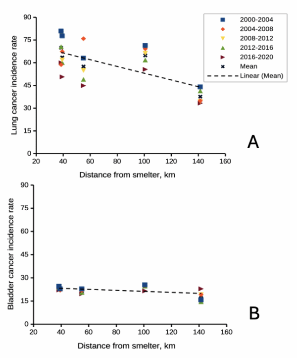
Figure 2. County cancer rates (A, lung and bronchial; B, bladder) from 2000 – 2020 vs distance in kilometers from ASARCO smelter, Ruston, WA. Data compiled from Washington Tracking Network (WTN). The counties were King (55 km), Kitsap (39.28 km), Pierce (38.48 km), San Juan ( 141.43 km), Snohomish (100.73 km), and Spokane (385.34 km).
If this scenario seems plausible, I hope you immediately recognize it as a case of confirmation bias (see Chapter 2.6). Putting aside for a moment the different arsenic species, each with different LD50 (the lethal dose needed to kill half the population — see Chapter 20.10), the difficulty ascribing arsenic as a causal agent for my Dad’s cancer is that many other exposures happened simultaneously. For example, indoor carpets are a primary source of several volatile organic compounds (Haines et al 2020). Prior to 1980 carpets may have included formaldehyde and other known carcinogenic agents. Dad commuted by car between work and home — with a ferry ride between — for decades (until the early 1990s), routinely traveling heavily congested roadways, this during the years prior to and the early years of the Clean Air Act of Environmental Protection Agency of the United States (it wasn’t until 1981 that new cars met EPA emission standards: Clean Air Act timeline here). Thus, all commuters including my Dad were exposed to gasoline combustion emissions, many known to be carcinogenic (Parent et al 2007). Moreover, a limited study by Public Health of Seattle and King County (2001) found rates of cancer on Vashon between 1980 and 1988 were similar to other areas in King County.
Summary.
It’s easy to fall into the trap that experiments — and by extension meta-analysis and systematic reviews — are the best tools offered by science for developing knowledge about the world, and other approaches suffer by comparison. But after even a bit of reflection, we should recognize that it can’t be that simple. While we now “know” tobacco cigarette smoking increases lung cancer risk, and many experiments with animal models convincingly show the link (eg, Hutt et al 2005), no human experiment in the strict sense, ie, prospective, randomized control trial, has ever been conducted (hint: it would be unethical, see discussion in Allmark and Tod 2016). Instead, the accumulated evidence from observational studies on exposures of different populations over the years overwhelmingly points to smoking as a leading risk factor (cause) of lung and other cancers — an example of Hill’s guidelines of causality. We end with a quote:
RCTs can play a role in building scientific knowledge and useful predictions but they can only do so as part of a cumulative program, combining with other methods, including conceptual and theoretical development, to discover not ‘what works’, but ‘why things work’ (p 2, Deaton and Cartwright 2017).
Questions.
.
- Write up three learning outcomes for this page. Hint: Point your favorite generative AI to this page and ask for help.
- Was my Dad’s lung cancer attributable to his 40 years plus exposure to soil arsenic (he’s a non-smoker)? How should we approach this question?
- In Diener et al (2006), the authors concluded that because acupuncture lacks side-effects that may occur with standard therapies acupuncture may be a good choice for patients seeking relief from migraine. Do you agree with the authors?
- Ethical standards evolve with time. An ongoing debate in research is whether and how placebos are to be used in human subjects research. Placebos are a means to establish controls in a study so that effects may be attributed to the active treatment. The “gold standard” of clinical trials is considered to be the randomized double-blind design — neither the patient-subject nor the researchers know who receives the placebo or the treatment. Following review of the WHO report on Use of Placebos in Vaccine Trials, pick one study and evaluate whether or not the decision to use placebos was warranted in your opinion.
- I searched PUBMED for “double-blind” by decade and found the following results (August 2018) (Table 1). Open R and/or R Commander and create two variables, then generate a scatter plot. Describe the shape of the relationship between number of publications citing “double-blind” and time (eg, 1950 – 1959, 1960 – 1969, and so on).
| Decade | Publications |
|---|---|
| 1950 | 60 |
| 1960 | 995 |
| 1970 | 7184 |
| 1980 | 24737 |
| 1990 | 39643 |
| 2000 | 53965 |
| 2010 | 69265 |
- Here’s one way to enter this data into R. At the R prompt (or in the R Script window of R Commander), create two variables,
DecadeandPubsDecade <- c(seq(1950, 2020, by=10))Pubs <- c(59,995,7161,24728,39670,54011,57043)Make an XY scatter plotplot(Decade,Pubs) - Repeat the PUBMED search as above but search for “placebo”. Make a table like the one above and provide a scatterplot of your results.
- Is the concept of a placebo relevant if the subjects in your experiment are yeast cells, not humans?
- Similarly, if your subjects are yeast cells, how does the concept of performing experiments “blind” apply?
- Ethical standards change with time. An ongoing debate in research is whether and how placebos are to be used in human subjects research.
- If placebos are so important, why is their use a concern in clinical trials?
- Following review of the WHO report on Use of Placebos in Vaccine Trials (see Readings below), pick one study and evaluate whether or not the decision to use placebos was warranted in your opinion.
R notes for question 5:
<-is an assignment operator (assignOP); everything to the right of<-is assigned to the object named to the left of the<-operator. You can instead use=in place of<-, but because=is also used in other contexts besides assignment, a quick look at blogs by data scientists will find a preference to use<-for clarity and consistency.c()“combines” arguments into a vector.seq()is used to generate a sequence of numbers between a lower and an upper limit; ifby = nis included, the sequence will be increased by the value n. If omitted, then the sequence is increased by 1.
Quiz Chapter 2.4
Chapter 2 contents.
.
- Introduction
- Why biostatistics?
- Why do we use R Software?
- A brief history of (bio)statistics
- Experimental Design and rise of statistics in medical research
- Scientific method and where statistics fits
- Statistical reasoning
- Chapter 2 – References and suggested reading