9.1 – Chi-square test: Goodness of fit
Introduction
We ask about the “fit” of our data against predictions from theory, or from rules that set our expectations for the frequency of particular outcomes drawn from outside the experiment. Three examples to illustrate goodness of fit, GOF,  , A, B, and C follow.
A. For example, for a toss of a coin, we expect heads to show up 50% of the time. Out of 120 tosses of a fair coin, we expect 60 heads, 60 tails. Thus, our null hypothesis would be that heads would appear 50% of the time. If we observe 70 heads in an experiment of coin tossing, is this a significantly large enough discrepancy to reject the null hypothesis?
B. For example, simple Mendelian genetics makes predictions about how often we should expect particular combinations of phenotypes in the offspring when the phenotype is controlled by one gene, with 2 alleles and a particular kind of dominance.
For example, for a one locus, two allele system (one gene, two different copies like R and r) with complete dominance, we expect the phenotypic (what you see) ratio will be 3:1 (or  round,
 wrinkle). Our null hypothesis would be that pea shape will obey Mendelian ratios (3:1). Mendel’s round versus wrinkled peas (RR or Rr genotypes give round peas, only rr results in wrinkled peas).
Thus, out of 100 individuals, we would expect 75 round and 25 wrinkled. If we observe 84 round and 16 wrinkled, is this a significantly large enough discrepancy to reject the null hypothesis?
C. For yet another example, in population genetics, we can ask whether genotypic frequencies (how often a particular copy of a gene appears in a population) follow expectations from Hardy-Weinberg model (the null hypothesis would be that they do).
This is a common test one might perform on DNA or protein data from electrophoresis analysis. Hardy-Weinberg is a simple quadratic expansion:
If p = allele frequency of the first copy, and q = allele frequency of the second copy, then p + q = 1,
Given the allele frequencies, then genotypic frequencies would be given by 1 = p2 + 2pq + q2.
Deviations from Hardy-Weinberg expectations may indicate a number of possible causes of allele change (including natural selection, genetic drift, migration).
Thus, if a gene has two alleles,  and
 , with the frequency for ,
 and for ,
 (equivalently q = 1 – p) in the population, then we would expect 36
 , 16
 , and 48
 individuals. (Nothing changes if we represent the alleles as A and a, or some other system, eg, dominance/recessive.)
Question. If we observe the following genotypes: 45 individuals, 34 individuals, and 21 individuals, is this a significantly large enough discrepancy to reject the null hypothesis?
Table 1. Summary of our Hardy Weinberg question
| Genotype | Expected | Observed | O – E |
| aa | 70 | 45 | -25 |
| aa’ | 27 | 34 | 7 |
| a’a’ | 3 | 21 | 18 |
| sum | 100 | 100 | 0 |
Recall from your genetics class that we can get the allele frequency values from the genotype values, eg,
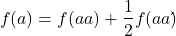
We call these chi-square tests, tests of goodness of fit. Because we have some theory, in this case Mendelian genetics, or guidance, separate from the study itself, to help us calculate expected values in a chi-square test.
Note 1: The idea of fit in statistics can be reframed as how well does a particular statistical model fit the observed data. A good fit can be summarized by accounting for the differences between the observed values and the comparable values predicted by the model.
Note also for our coin toss example, goodness of fit isn’t exactly proper terminology — afterall the test is equal probability of the two outcomes, not whether we have match between an observed distribution and an expected distribution (true statement if we add “follows a binomial distribution”).
 goodness of fit
For k groups, the equation for the chi-square test may be written as
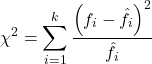
where fi is the frequency (count) observed (in class i) and fi<hat> is the frequency (count) expected if the null hypothesis is true, sum over all k groups. Alternatively, here is a format for the same equation that may be more familiar to you… ?
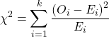
where Oi is the frequency (count) observed (in class i) and Ei is the frequency (count) expected if the null hypothesis is true.
The degrees of freedom, df, for the GOF are simply the number of categories minus one, k – 1.
Explaining GOF
Why am I using the phrase “goodness of fit?” This concept has broad use in statistics, but in general it applies when we ask how well a statistical model fits the observed data.
At least for the chi-square test it is simple to see how the test statistic increases from zero as the agreement between observed data and expected data depart, where zero would be the case in which all observed values for the categories exactly match the expected values.
The goodness of fit test is designed to evaluate whether or not your data agree with a theoretical expectation (there are additional ways to think about this test, but this is a good place to start). Let’s take our time here and work with an example. The other type of chi-square problem or experiment is one for the many types of experiments in which the response variable is discrete, just like in the GOF case, but we have no theory to guide us in deciding how to obtain the expected values. We can use the data themselves to calculate expected values, and we say that the test is “contingent” upon the data, hence these types of chi-square tests are called contingency tables.
You may be a little concerned at this point that there are two kinds of chi-square problems, goodness of fit and contingency tables. We’ll deal directly with contingency tables in the next section, but for now, I wanted to make a few generalizations.
- Both goodness of fit and contingency tables use the same chi-square equation and analysis. They differ in how the degrees of freedom are calculated.
- Thus, what all chi-square problems have in common, whether goodness of fit or contingency table problems
- You must identify what types of data are appropriate for this statistical procedure? Categorical (nominal data type).
- As always, a clear description of the hypotheses being examined.
For goodness of fit chi-square test, the most important type of hypothesis is called a Null Hypothesis: In most cases the Null Hypothesis (HO) is “no difference” “no effect”…. If HO is concluded to be false (rejected), then an alternative hypothesis (HA) will be assumed to be true. Both are specified before tests are conducted. All possible outcomes are accounted for by the two hypotheses.
From above, we have
- A. HO: Fifty out of 100 tosses will result in heads.
- HA: Heads will not appear 50 times out of 100.
- B. HO: Pea shape will equal Mendelian ratios (3:1).
- HA: Pea shape will not equal Mendelian ratios (3:1).
- C. HO: Genotypic frequencies will equal Hardy-Weinberg expectations.
- HA: Genotypic frequencies will not equal Hardy-Weinberg expectations
Assumptions: In order to use the chi-square, there must be two or more categories. Each observation must be in one and only one category. If some of the observations are truly halfway between two categories then you must make a new category (eg, low, middle, high) or use another statistical procedure. Additionally, your expected values are required to be integers, not ratio. The number of observed and the number of expected must sum to the same total.
The chi-square test is a good example of such tests, and we will encounter other examples too. Another common goodness of fit is the coefficient of determination, which will be introduced in linear regression sections (see Chapter 17.7 – Regression model fit). Still other examples are the likelihood ratio test (LRT), Akaike Information Criterion (AIC), and Bayesian Information Criterion (BIC), which are all used to assess fit of models to data. (See Graffelman and Weir [2018] for how to use AIC in the context of testing for Hardy Weinberg equilibrium.)
The likelihood ratio test is used to compare the goodness of fit of two hierarchically nested models to determine if a more complex model provides a significantly better fit to the data. It does this by forming a ratio of the likelihood of the data under the two models (the simpler “null” model and the more complex “alternative” model). A small ratio suggests the simpler model is a poor fit, while a value close to one indicates the added complexity is not statistically significant. AIC (and BIC) is a measure of relative fit — it balances goodness of fit and model complexity: A lower AIC suggests a better model by finding the optimal trade-off between fitting the data well and keeping the model simple. A model that is too complex will have a higher AIC than a simpler model with a nearly as good fit.
We use LRT, AIC and BIC when we talk about selecting best regression models (see Chapter 17.7 – Regression model fit). However, as we discuss the concept of comparing models, we need to distinguish between the concept of model choice — methods used to select a best model from competing options and estimating the “goodness of fit” of a single model.
How well does data fit the prediction?
Frequentist approach interprets the test as, how well does the data fit the null hypothesis,  ? When you compare data against a theoretical distribution (eg, Mendel’s hypothesis predicts the distribution of progeny phenotypes for a particular genetic system), you test the fit of the data against the model’s predictions (expectations). Recall that the Bayesian approach asks how well does the model fit the data?
Table 2. A. 120 tosses of a coin, we count heads 70/120 tosses.
| Expected | Observed | |
| Heads | 60 | 70 |
| Tails | 60 | 50 |
| n | 120 | 120 |

Table 3. B. A possible Mendelian system of inheritance for a one gene, two allele system with complete dominance, observe the phenotypes.
| Expected | Observed | |
| Round | 75 | 84 |
| Wrinkled | 25 | 16 |
| n | 100 | 100 |

Table 4. C. A possible Mendelian system of inheritance for a one gene, two allele system with complete dominance, observe the phenotypes.
| Expected | Observed | |
| p2 | 70 | 45 |
| 2pq | 27 | 34 |
| q2 | 3 | 21 |
| n | 100 | 100 |

For completeness, instead of a goodness of fit test we can treat this problem as a test of independence, a contingency table problem. We’ll discuss contingency tables more in the next section, but or now, we can rearrange our table of observed genotypes for problem C, as a 2X2 table
Table 5. Problem C reported in 2X2 table format.
| Maternal a’ | Paternal a’ | |
| Maternal a | 45 | 17 |
| Paternal a | 17 | 21 |
The contingency table is calculated the same way as the GOF version, but the degrees of freedom are calculated differently: df = number of rows – 1 multiplied by the number of columns – 1.

Thus, for a 2X2 table the df are always equal to 1.
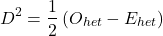
Note that the chi-square value itself says nothing about how any discrepancy between expectation and observed genotype frequencies come about. Therefore, one can rearrange the equation to make clear where deviance from equilibrium, D, occur for the heterozygote (het). We have

where D2 is equal to
φ coefficient
The chi-square test statistic and its inference tells you about the significance of the association, but not the strength or effect size of the association. Not surprisingly, Pearson (1904) came up with a statistic to quantify the strength of association between two binary variables, now called the φ (phi) coefficient. Like the Pearson product moment correlation, the φ (phi) coefficient takes values from -1 to +1.
Note 2: Pearson termed this statistic the mean square contingency coefficient. Yule (1912) termed it the phi coefficient. The correlation between two binary variables is also called the Mathews Correlation Coefficient or MCC (Mathews 1975), which is a common classification tool in machine learning.
The formula for the absolute value of φ coefficient is

Thus, for A, B, and C examples, φ coefficient was 0.167, 0.190, and 0.771. Thus, only weak associations in examples A and B, but strong association in C. We’ll provide a formula to directly calculate φ coefficient from the cells of the table in 9.2 – Chi-square contingency tables.
Carry out the test and interpret results
What was just calculated? The chi-square, , test statistic.
Just like t-tests, we now want to compare our test statistic against a critical value — calculate degrees of freedom (df = k – 1, k equals the numbers of categories), and set a rejection level, Type I error rate. We typically set the Type I error rate at 5%. A table of critical values for the chi-square test is available in Appendix Table Chi-square critical values.
Obtaining Probability Values for the goodness-of-fit test of the null hypothesis:
As you can see from the equation of the chi-square, a perfect fit between the observed and the expected would be a chi-square of zero. Thus, asking about statistical significance in the chi-square test is the same as asking if your test statistic is significantly greater than zero.
The chi-square distribution is used and the critical values depend on the degrees of freedom. Fortunately for and other statistical procedures we have Tables that will tell us what the probability is of obtaining our results when the null hypothesis is true (in the population).
Here is a portion of the chi-square critical values for probability that your chi-square test statistic is less than the critical value (Fig 1).
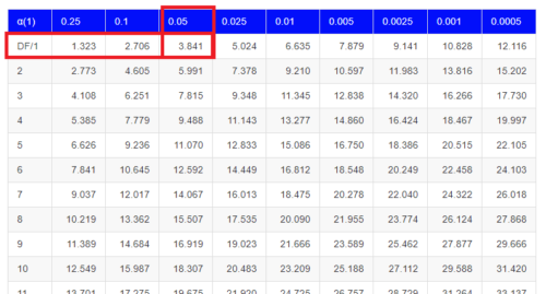
Figure 1. A portion of critical values of the chi-square at alpha 5% for degrees of freedom between 1 and 10. A more inclusive table is provided in the Appendix, Table of Chi-square critical values.
For the first example (A), we have df = 2 – 1 = 1 and we look up the critical value corresponding to the probability in which Type I = 5% are likely to be smaller iff (“if and only if”) the null hypothesis is true. That value is 3.841; our test statistic was 3.330, and therefore smaller than the critical value: so we do not reject the null hypothesis.
Interpolating p-values
How likely is our test statistic value of 3.333 and the null hypothesis was true? (Remember, “true” in this case is a shorthand for our data was sampled from a population in which the HW expectations hold). When I check the table of critical values of the chi-square test for the “exact” p-value, I find that our test statistic value falls between a p-value 0.10 and 0.05 (represented in the table below). We can interpolate
Note 3: Interpolation refers to any method used to estimate a new value from a set of known values. Thus, interpolated values fall between known values. Extrapolation on the other hand refers to methods to estimate new values by extending from a known sequence of values.
Table 6. Interpolated p-value for critical value not reported in chi-square table.
| statistic | p-value |
| 3.841 | 0.05 |
| 3.333 | x |
| 2.706 | 0.10 |
If we assume the change in probability between 2.706 and 3.841 for the chi-square distribution is linear (it’s not, but it’s close), then we can do so simple interpolation.
We set up what we know on the right hand side equal to what we don’t know on the left hand side of the equation,

and solve for x. Then, x is equal to 0.0724
R function pchisq() gives a value of p = 0.0679. Close, but not the same. Of course, you should go with the result from R over interpolation; we mention how to get the approximate p-value by interpolation for completeness, and, in some rare instances, you might need to make the calculation. Interpolating is also a skill used to provide estimates where the researcher needs to estimate (impute) a missing value.
Interpreting p-values
This is a pretty important topic, so much so that we devote an entire section to this very problem — see 8.2 – The controversy over proper hypothesis testing. If you skipped the chapter, but find yourself unsure how to interpret the p-value, then please go back to Ch 8.2. OK, that commercial message, what does it mean to “reject the chi-square null hypothesis?” These types of tests are called goodness of fit in the following sense — if your data agree with the theoretical distribution, then the difference between observed and expected should be very close to zero. If it is exactly zero, then you have a perfect fit. In our coin toss case, if we say that the ratio of heads:tails do not differ significantly from the 50:50 expectation, then we accept the null hypothesis.
You should try the other examples yourself! A hint, the degrees of freedom are one (1) for example B and two (2) for example C.
R code
Printed tables of the critical values from the chi-square distribution, or for any statistical test for that matter are fine, but with your statistical package R and Rcmdr, you have access to the critical value and the p-value of your test statistic simply by asking. Here’s how to get both.
First, let’s get the critical value.
Rcmdr: Distributions → Continuous distributions → Chi-squared distribution → Chi-squared quantiles (Fig 2).
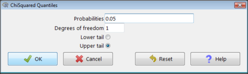
Figure 2. R Commander menu for Chi-squared quantiles.
I entered “0.05” for the probability because that’s my Type I error rate α. Enter “1” for Degrees of freedom, then click “upper tail” because we are interested in obtaining the critical value for α. Here’s R’s response when I clicked “OK.”
qchisq(c(0.05), df=1, lower.tail=FALSE)
[1] 3.841459
Next, let’s get the exact P-value of our test statistic. We had three from three different tests:  for the coin-tossing example,
 for the pea example, and
 for the Hardy-Weinberg example.
Rcmdr: Distributions → Continuous distributions → Chi-squared distribution → Chi-squared probabilities… (Fig 3).
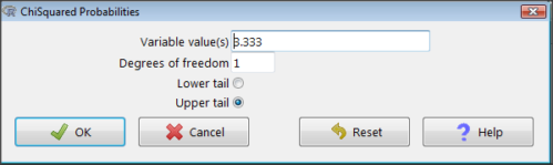
Figure 3. R Commander menu for Chi-squared probabilities.
I entered “3.333” because that is one of the test statistics I want to calculate for probability and “1” for Degrees of freedom because I had k – 1 = 1 df for this problem. Here’s R’s response when I clicked “OK.”
pchisq(c(3.333), df=1, lower.tail=FALSE)
[1] 0.06790291
I repeated this exercise for I got  ; for I got
 .
Nice, right? Saves you from having to interpolate probability values from the chi-square table.
3. How to get the goodness of fit in Rcmdr.
R provides the goodness of fit (the command is chisq.text()), but Rcmdr thus far does not provide a menu option to link to the function. Instead, R Commander provides a menu for contingency tables, which also is a chi-square test, but is used where no theory is available to calculate the expected values (see Chapter 9.2). Thus, for the goodness of fit chi-square, we will need to bypass Rcmdr in favor of the script window. Honestly, other options are as quick or quicker: calculate by hand, use a different software (eg, Microsoft Excel), or many online sites provide JavaScript tools.
So how to get the goodness of fit chi-square while in R? Here’s one way. At the command line, type
chisq.test (c(O1, O2, ... On), p = c(E1, E2, ... En))
where O1, O2, … On are observed counts for category 1, category 2, up to category n, and E1, E2, … En are the expected proportions for each category. For example, consider our Heads/Tails example above (problem A).
In R, we write and submit
chisq.test(c(70,30),p=c(1/2,1/2))
R returns
Chi-squared test for given probabilities.
data: c(70, 30)
X-squared = 16, df = 1, p-value = 0.00006334
Easy enough. But not much detail — details are available with some additions to the R script. I’ll just link you to a nice website that shows how to add to the output so that it looks like the one below.
mike.chi <- chisq.test(c(70,30),p=c(1/2,1/2))
Let’s explore one at time the contents of the results from the chi square function.
names(mike.chi)   #The names function
[1] "statistic" "parameter" "p.value" "method" "data.name" "observed"
[7] "expected" "residuals" "stdres"
Now, call each name in turn.
mike.chi$residuals
[1] 2.828427 -2.828427
mike.chi$obs
[1] 70 30
mike.chi$exp
[1] 50 50
Note 4: “residuals” here simply refers to the difference between observed and expected values. Residuals are an important concept in regression, see Ch17.5
And finally, let’s get the summary output of our statistical test.
mike.chi
Chi-squared test for given probabilities.
data: c(70, 30)
X-squared = 16, df = 1, p-value = 6.334e-05
GOF and spreadsheet apps
Easy enough with R, but it may even easier with other tools. I’ll show you how to do this with spreadsheet apps and with and online at graphpad.com.
Let’s take the pea example above. We had 16 wrinkled, 84 round. We expect 25% wrinkled, 75% round.
Now, with R, we would enter
chisq.test(c(16,80),p=c(1/4,3/4))
and the R output
Chi-squared test for given probabilities
data: c(16, 80)
X-squared = 3.5556, df = 1, p-value = 0.05935
Microsoft Excel and the other spreadsheet programs (Apple Numbers, Google Sheets, LibreOffice Calc) can calculate the goodness of fit directly; they return a P-value only. If the observed data are in cells A1 and A2, and the expected values are in B1 and B2, then use the procedure =CHITEST(A1:A2,B1:B2).
Table 7. A spreadsheet with formula visible.
| A | B | C | D | |
| 1 | 80 | 75 | ||
| 2 | 16 | 25 | =CHITEST(A1:A2,B1:B2) |
The P-value (but not the Chi-square test statistic) is returned. Here’s the output from Calc.
Table 8. Spreadsheet example from Table 7 with calculated P-value.
| A | B | C | D | |
| 1 | 80 | 75 | ||
| 2 | 16 | 25 | 0.058714340077662 |
You can get the critical value from MS Excel (=CHIINV(alpha, df), returns the critical value), and the exact probability for the test statistic =CHIDIST(x,df), where x is your test statistic. Putting it all together, a general spreadsheet template for goodness of fit calculations calculations of test statistic and p-value might look like
Table 9. Spreadsheet template with formula to calculate chi-square goodness of fit on two groups.
| A | B | C | D | E | |
| 1 | f1 | 0.75 | |||
| 2 | f2 | 0.25 | |||
| 3 | N | =SUM(A5,A6) |
|||
| 4 | Obs | Exp | Chi.value | Chi.sqr | |
| 5 | 80 | =B1* |
=((A5-B5)^2)/B5 |
=SUM(C5,C6) |
|
| 6 | 16 | =B2* |
=((A6-B6)^2)/B6 |
=CHIDIST(D5, COUNT(A5:A6-1) |
|
| 7 | |||||
| 8 |
 3
Microsoft Excel can be improved by writing macros, or by including available add-in programs, such as the free PopTools, which is available for Microsoft Windows 32-bit operating systems only.
Another option is to take advantage of the internet — again, many folks have provided java or JavaScript-based statistical routines for educational purposes. Here’s an easy one to use www.graphpad.com.
In most cases, I find the chi-square goodness-of-fit is so simple to calculate by hand that the computer is redundant.
Questions
1. A variety of p-values were reported on this page with no attempt to reflect significant figures or numbers of digits (see Chapter 8.2). Provide proper significant figures and numbers of digits as if these p-values were reported in a science journal.
- 0.0724
- 0.0679
- 0.03766692
- 0.004955794
- 0.00006334
- 6.334e-05
- 0.05935
- 0.058714340077662
2. For a mini bag of M&M candies, you count 4 blue, 2 brown, 1 green, 3 orange, 4 red, and 2 yellow candies.
- What are the expected values for each color?
- Calculate using your favorite spreadsheet app (eg, Numbers, Excel, Google Sheets, LibreOffice Calc)
- Calculate using R (note R will reply with a warning message that the “Chi-squared approximation may be incorrect”; see 9.2 Yates continuity correction)
- Calculate using Quickcalcs at graphpad.com
- Construct a table and compare p-values obtained from the different applications
3. CYP1A2 enzyme involved with metabolism of caffeine. Folks with C at SNP rs762551 have higher enzyme activity than folks with A. Populations differ for the frequency of C. Using R or your favorite spreadsheet application, compare the following populations against global frequency of C is 33% (frequency of A is 67%).
- 286 persons from Northern Sweden: f(C) = 26%, f(A) = 73%
- 4532 Native Hawaiian persons: f(C) = 22%, f(A) = 78%
- 1260 Native American persons: f(C) = 30%, f(A) = 70%
- 8316 Native American persons: f(C) = 36%, f(A) = 64%
- Construct a table and compare p-values obtained for the four populations.
Quiz Chapter 9.1
Chi-square test: Goodness of fit
Chapter 9 contents
5.1 – Experiments
How to put an experiment together
With the background behind us, we outline a designed experiment. Readers may wish to review concepts presented previously, in
- Chapter 2.4: Experimental design and rise of statistics in medical research.
- Chapter 3.4 – Estimating parameters
- Chapter 3.5 – Statistics of error
Experiments have the following elements
- Define a reference population.
- All patients with similar angina symptoms — shortness of breath, chest pain, dizziness — but who have not suffered a heart attack, or myocardial infarction (Wu et al 2017);
- All adult frogs in a pond near industrial waste runoff (eg, Sowers et al 2009).
- Define sample unit from the reference population (eg, as many patients as can be screened by the physician are recruited; all frogs visible to the biologist are captured).
- Design sampling scheme from population (eg, random sampling vs. convenience/haphazard sampling).
- Agree on the primary outcome or endpoint to be measured and whether additional secondary outcomes are to be observed and collected.
- For the patients with similar symptoms, we follow
- For the frogs, we count adults with developmental malformations.
- Separate the sample into groups so that comparisons can be made
- We may be tempted to provide the same treatment and follow the group for improvement — that is the clinically valid approach; to be an experiment, we would use random assignment of individuals to one of two groups — half will receive a placebo, half will receive a beta blocker;,
- The frog example doesn’t follow this scheme — the event has already occured, it’s an observational study.
- Devise a way to exclude or distinguish from the possible explanations, or alternative hypotheses.
- eg, for the physician, she will record how many of her patients fail to respond to treatment;
- for the biologist, noting presence or absence of parasites between the normal and abnormal frog defines the groups).
Note 1: The studies cited are examples of work done on similar problems, they are not offered to evaluate or critique any research efforts that were done or described in these reports.
The frog study, as described by me for pedagological purposes, lacks any design elements that would allow for a test of the hypothesis that industrial runoff causes developmental malformations in frogs — I’m not saying or implying anything about the actual studies!
A basic experimental design looks like this.
- One treatment, with two levels (eg, a control group and an experimental group)
- A collection of individuals recruited from a defined population, esp. by random sampling.
- Random assignment of multiple individuals to one of the two treatment levels.
- The treatments are applied to each individual in the study.
- A measure of response (the primary outcome) and additional features (secondary outcomes) are recorded for each individual.
Of course, there are other considerations, and by now, students reading this text should be able to identify what is missing from the list. (See quiz questions.)
Contrast with design of observational studies
Importantly, for observational studies, no matter how sophisticated the equipment used to measure the outcome variable(s), key steps outlined above are missing. Researchers conducting observational studies do not control allocation of subjects to treatment groups (steps 4 and 3 in the two above lists, respectively). Instead, they may use case-control approaches, where individuals with (case) and without (control) the condition (eg, lung cancer) are compared with respect to some candidate risk factor (eg, smoking). Both case and control groups likely have members who smoke, but if there is an association between smoking and lung cancer, then more smokers will be in the case group compared to the control group.
A cohort study, also a form of observational study, is similar to case-control except that the outcome status is not known. A cohort study includes, in our example, smokers and non smokers who share other characteristics: age, medical history, etc. The other kind of design you will see is the cross-sectional study. Cross-sectional studies are descriptive studies, and, therefore also observational. Primary outcomes along with additional characteristics and outcomes are measured for a representative subsample, or perhaps even an entire population. Cross-sectional studies are used to absolute and relative risk rates. In ecology and evolutionary biology cross sectional studies are common, eg, comparisons of species for metabolic rate (Darveau et al 2005) or life history traits (Jennings et al 1998), and specialized statistical approaches that incorporate phylogenetic information about the species are now the hallmark of these kinds of studies.
A word on outcomes of an experiment. Experiments should be designed to address an important question. The outcomes the researcher measures should be directly related to the important question. Thus, in the design of clinical trials, researchers distinguish between primary and secondary outcomes or endpoints. In educational research the primary question is whether or not students exposed to different teaching styles (eg, lecture-style or active-learning approaches) score higher on an knowledge-content exams. The primary outcome would be the scores on the exams; many possible secondary outcomes might be collected including student’s attitudes towards the subject or perceptions on how much they have learned.
Note 3: While it’s logical to include secondary outcomes — they may offer support or complement the primary results — there needs to be caution in interpreting the test results of multiple secondary outcomes. By definition, the study is designed to test hypothesis about the primary or main outcome. While there are a number of concerns about testing secondary outcomes, from a statistical point of view, the study may lack the sample size — the power, see Chapter 11 — Power analysis — to test many additional hypotheses without the risk of increasing chance of false positives because of the multiple comparisons problem. We address this scenario in Chapter 12.1 – The need for ANOVA.
About Primary and Secondary Outcomes.
Consider a evolutionary physiology project on species differences and effects of body size on burst running speed of terrestrial lizards (eg, Bauwens et al 1995; Dohm et al 1998; Labonte et al 2024). Our independent variables, the things we believe influence running performance — and therefore we wish to control for — species, body size, core body temperature, body condition, race quality (see cited papers for these and other examples).
What do we measure? What are the likely primary vs. secondary outcomes for a this kind of project?
Primary outcomes are the direct, definitive measures of maximal locomotor performance. Examples may include
- Maximum Burst Speed: The absolute highest velocity achieved by the lizard over a short distance or time interval (eg, across a 0.5-meter interval).
- Maximum Acceleration: The highest rate of speed change during the start of the burst or during a sudden sprint increase.
- Stride Length: The physical distance covered during a single full stride cycle at maximum speed.
- Stride Frequency: The number of strides taken per second at maximum speed.
And what other measures may be of interest — secondary outcomes — those that may help explain why or how the primary performance metrics change across the independent variables. To list a few,
- Stance and Swing Duration: The individual time durations spent with feet on the ground (stance) vs. in the air (swing).
- Gait Transition Thresholds: The speed at which a lizard shifts from a walk/trot to a high-speed gallop or bipedal running (if applicable to the species).
- Fatigue Rate: The decline in burst speed across successive trials or over a sustained treadmill run.
- Trial-to-Trial Repeatability: The statistical consistency (intraclass correlation coefficient) of a lizard’s performance across multiple bursts.
In a prospective cohort study, we may track participants over time to observe how baseline factors predict the development or worsening of type 2 diabetes (eg, Gao et al 2026). Progression over a two year followup would be measured by incident clinical events or the longitudinal rate of change in biomarkers. Possible primary outcomes are
- Glycated Hemoglobin (HbA1c): A biomarker reflecting average blood glucose levels over the past 2 to 3 months (glycemic control).
- Fasting Plasma Glucose (FPG): Glucose concentration in the blood after an overnight fast (acute baseline glycemic regulation).
- T2D Complication Stage: A clinical score or categorization indicating the presence and severity of microvascular or macrovascular damage.
Secondary outcomes may include
- Fasting Lipid Profile
- C-Reactive Protein
- Body Mass Index
- Estimated Glomerular Filtration Rate
If one or more primary outcomes are significant, this reveals whether an intervention or exposure (like a vegan diet or income level) changes the clinical course of Type 2 Diabetes. Secondary outcomes are critical for explaining how and why it happens. Secondary outcomes provide mechanistic context.
Some caution is warranted — imagine if, after conducting the study, we find diet, age, or income did not statistically affect your primary outcome, but did significantly alter a secondary outcome (eg, improved lipid profiles). What to report? We state in your Abstract and Discussion that the study failed to meet its primary objective, and that any significant secondary findings are exploratory. We cannot claim that a diet “successfully manages diabetes progression” based solely on a secondary marker (cf discussion and suggsted guidelines in Butcher et al 2022).
Example of an experiment.
We’ll work through a familiar example. The researcher is given the task to design a study to test the efficacy in reducing tension headache symptoms by a new pain reliever. There are many possible outcomes: blurry vision, duration, frequency, nausea, need for and response to pain medication, and level of severity (Mayo Clinic). The drug is packaged in a capsule and a placebo is designed that contains all ingredients except the new drug. Forty subjects with headaches are randomly selected from a population of headache sufferers. All forty subjects sign the consent form and agree to be part of the study. The subjects also are informed that while they are participating in the research study on a new pain reliever, each subject has a 50-50 chance of receiving a placebo and not the new drug. The researcher then randomly assigns twenty of the subjects to receive the drug treatment and twenty to receive the placebo, places either a placebo pill of the treatment pill into a numbered envelope and gives the envelopes to a research partner. The partner then gives the envelopes to the patients. Both patients and the research partner are kept ignorant of the assignment to treatment.
We can summarize this most basic experimental design in a table, Table 1.
Table 1. Simple formulation of a 2X2 experiment (aka 2×2 contingency table).
| Did the subject get better? | ||||
|---|---|---|---|---|
| Yes | No | Row totals | ||
| Subject received the treatment |
Yes | a | b | a + b |
| No | c | d | c + d | |
| Column totals | a + c | b + d | N | |
where N is the total number of subjects, a is number of subjects who DID receive the treatment AND got better, c is number of subjects who DID NOT receive the treatment, but DID get better, b is number of subjects who DID receive the treatment and DID NOT get better, and d is number of subjects who DID NOT receive the treatment and DID NOT get better.
Note 4: We owe Karl Pearson (1904) for the concepts of contingency — that membership in a (or b, c, or d for that matter) is a deviation from any chance association or independent probability (Chapter 6) — and the contingency table. Contingency is an important concept in classification and is central to machine learning in data science (Michie et al 1995). We return at some length to contingency and how to analyze contingency tables in Chapter 7 and Chapter 9.2.
By convention, the standard format for an epidemiological 2×2 contingency table organizes exposure on the rows and disease outcome on the columns as follows:
- Rows (Exposure): The top row represents Exposed / Treatment (Yes), and the bottom row represents Non-exposed / Control (No).
- Columns (Outcome): The left column represents Disease / Case (Yes), and the right column represents No Disease / Control (No). See Chapter 7.
And our basic expectation is that we are testing whether or not treatment levels were associated with subjects “getting better” as measured on some scale.
One possible result of the experiment, although unlikely, all of the negative outcomes are found in the group that did not receive the treatment (Table 2).
Table 2. One possible outcome of our 2X2 experiment.
| Subject improved | |||
|---|---|---|---|
| Yes | No | ||
| Subject received the treatment |
Yes | 20 | 0 |
| No | 0 | 20 | |
Results of an experiment probably won’t be as clear as in Table 2. Treatments may be effective, but not everyone benefits. Thus, results like Table 3 may be more typical.
Table 3. A more likely outcome of our 2X2 experiment.
| Subject improved | |||
|---|---|---|---|
| Yes | No | ||
| Subject received the treatment |
Yes | 7 | 13 |
| No | 2 | 18 | |
Must a control group always be included in an experiment?
To be an experiment, yes. However, it is not true that the control treatment must only be applied to separate, individual subjects. For example, a common experimental design would be repeated measures of an outcome, like behavior (eg, feeding response) before and after an intervention is applied. Thus, the individual is its own control or reference point. For example, Dohm et al (2008) measured feeding and locomotor behavior of adult toads (Rhinella marina, formerly Bufo marinus) prior to and after ozone exposure. We concluded that a single 4-h exposure to O3 depressed toad feeding behavior, but had little effect on voluntary locomotor behavior. Typically, the design randomly assigns individuals to the treatments — some individuals get the exposure first, then the control exposure second; others, again selected at random, receive the control exposure first, then the active exposure.
The within subjects design is an important method in biological research; these designs offer control for individual differences as confounding variables and require fewer participants compared to separate control group designs. This design is effective provided there is little risk of carryover effects; if the effects of a previous condition linger, then it may influence a participant’s response in subsequent conditions, confounding the results. For our study (Dohm et al 2008) we used a modified within-subjects design by employing a split plot design. We return to within-subjects designs in Chapter 14.4 – Randomized block design.
Questions
- When I updated this page in 2020, we were in our fifth month of the coronavirus pandemic of 2019-2020. Daily it seemed, we heard news about “promising coronavirus treatments,” but no study had at the time been published that would meets our considerations for a proper experiment. However, on May 1, 2020, the FDA issued an emergency use authorization for use of the antiviral drug remdesivir (Gilead), based on early results of clinical trials reported 29 April in The Lancet (Wang et al 2020). Briefly, their study included 158 treated with does of the antiviral drug and 79 provided with a placebo control. Both groups were treated otherwise the same. Improvement over 28 days was recorded: 62 improved with Placebo and 133 improved receiving dose of remdesivir.
- Using the background described on this page, list the information needed to design a proper experiment. Using your list, review the work described in The Lancet article and check for evidence that the trial meets these requirements.
- Create a 2×2 table with the described results from The Lancet article.
- Consider our hazel tea and copper solution experiment described in Chapter 3. The outcome variables (Tail length, tail percentage, Olive moment) are quantitative, not categorical. Create a table to display the experimental design.
- For the migraine example, identify elements of the design that conform to the randomized control trial design described in Chapter 2.4.
Quiz Chapter 5.1
Experiments
Chapter 5 contents
2.3 – A brief history of (bio)statistics
Foundations of biostatistics: key definitions.
.
Before discussing history and landmark moments in biostatistics, let’s start with basic definitions.
Bioinformatics is loosely defined as a discipline of biology primarily concerned with work involving large data sets (eg, databases), but a bioinformatician would not primarily be a statistician necessarily. Rather, a bioinformatician in addition to foundation in statistical and mathematical training would likely be fluent in at least one programming language and confident in use and design of databases.
Biostatistics, or biometry, then, refers to use of statistics in biology. Biostatistics encompasses application of statistical approaches to design, analyze, and interpret biological data collected through observation of use of experimentation. In turn, there are many broad disciplines or fields of specialty that trained biostatisticians may work.
Chance, the likelihood that a particular event will occur.
Data scientist, a very general label, is a person likely to work on “big data.” Big data may be loosely and inconsistently identified as access to large detailed and unstructured data sets such as visits and behavior within websites of tens of millions of Internet “hits” to a website like Amazon® or Google®. The data scientist would then be involved in extracting meaning from volumes of this data in a process called data mining. In the context of biology web sites like allele frequency aggregator at NCBI, which houses allele frequency information collected on human populations, the 1000 genome project, or any of the databases accessible at National Center for Biotechnology Information would constitute sources of big data for biological researchers.
Epidemiology refers to the statistics of patterns of and risk of disease in populations, particularly of humans and thus, an epidemiologist would also be considered to be a biostatistician. The statistics of epidemiology include all of the materials we will cover in this course, but perhaps if any particular analytical approach characterizes epidemiology, it would be survival analysis (review in Clark et al 2003) — in competition with compartment models to predict spread of communicable disease in populations (Brauer 2017).
Event, an outcome to which a probability is assigned.
Likelihood, the probable chance of occurrence of an event that has already occurred. Likelihood assesses how well a particular model or set of parameters explains observed data.
Probability, the chance that an event will occur in the future, given a known model or set of parameters.
Random or random chance. This is a good place to share a warning about vocabulary; statistics, like most of science, uses familiar words, but with refined and sometimes different meanings than our everyday usage. Consider our everyday use of random: “without definite aim, direction, rule, or method – subjects chosen at random” (Merriam-Webster online dictionary). In statistics, however, random refers to “an assignment of a numerical value to each possible outcome of an event” (Wikipedia, Eagle 2021). Thus, in statistics, random dictates a method of determining how likely a subject is to be included: If  represents the size of the population, then random sampling implies that each individual had
 chance of being selected. Thus, if
 , then each individual has a 1% (
 ) chance of selection. This is quite different from Merriam-Webster’s definition, in which no method is assumed. To a statistician, then, random as used in everyday conversation would imply haphazard sampling or convenience sampling from a population.
Statistics may be defined as the science of collecting, organizing, and interpreting data. Statistics is a branch of applied mathematics. Note that the word statistic is also used, but refers to a calculated quantity like the mean or standard deviation. A little confusing, but the context in which statistics or statistic is appropriate is usually not a major issue.
Note 1. Did you notice how the definitions for chance, likelihood, and probability were rather circular? Of the three, chance is more informal while both likelihood and probability are distinct concepts in statistics.
From dice games to data science: A brief history of statistics.
.
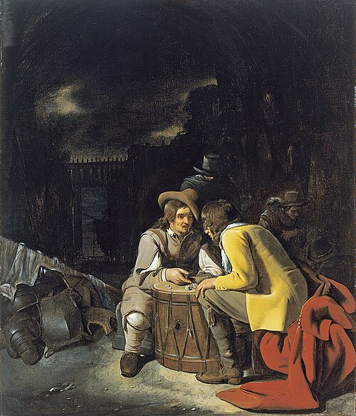
Figure 1. Soldiers playing dice, painting by Michiel Sweerts (1618–1664). Public domain image, https://commons.wikimedia.org/
The concepts of chance and probability, so crucial to statistical reasoning — because it allows us to interpret data when outcomes are inconsistent — were realized rather late in the history of mathematics. While people have been writing about applied and theoretical math for thousands of years, probability as a topic of interest by (Western) scholars seems to date only back to the late 17th century, beginning with letters written between Pierre de Fermat (1601-1665) and Blaise Pascal (1623 – 1662) and the substantial work on probability by Pierre-Simon Laplace (1749-1827). Often, research on probability developed under the watchful eyes of rich patrons more interested in gaming (sensu Fig 1), than to scientific applications. Work on permutations and combinations, essential for an understanding of probability, trace to India prior to Pascal’s work (Raju 2011).
The history of statistics goes back further if you allow for the dual use of the term statistics, both as a descriptor of the act of collecting data and as a systematic approach to the analysis of data. Prior to the 1700s, statistics was used in the sense of collection of data for use by the governments. It is not until the latter part of the 19th century that we see scholarship on statistical analytical techniques. Many of the statistical approaches we teach and use today were developed in the decades between 1880s and the 1930s. Work by Francis Galton (1822-1911), Karl Pearson (1857-1936), RA Fisher (1890-1962), Sewall Wright (1889-1988), Jerzy Neyman (1894-1981), Egon Pearson (1895-1980, Karl Pearson’s son), George EP Box (1919-2013) remains highly influential today.
Development of randomized controlled (clinical) trials, RCT, the “gold standard,” by the 1950s provides the strongest study design to evaluate the effectiveness of clinical or other kinds of interventions. The general features of RCT are (1) comparison among groups, with at least one control group, (2) randomization, and (3) blinding, where treatment options are concealed from the subjects (single-blind) and from those charged to assess the outcomes (double-blind). Sir Austin Bradford Hill (1887-1991) is generally credited with developing the RCT (Collier 2009, Matthews 2016), but we owe RA Fisher for randomization in experimental design. Hill (1965) is also known for Hill’s criteria of causality — nine principles that can be used to establish causal relationship between epidemiological (observational) evidence and disease. Chief among these nine principles are strength of the association (effect size) and consistent association (reproducibility), elements we return to often in our introduction to biostatistics.
Since the 1950s, there has been an explosion of developments in statistics, particularly as related to power of computer. These include use of resampling, simulation, and Monte Carlo methods (Harris 2010). Resampling — the creation of new samples based on a set of observed data — is a key innovation in statistics. Its use led to a number of innovative ways to estimate the precision of an estimate (see Chapter 3.4 and Chapter 19). Monte Carlo methods, or MCM, which involves resampling from a probability distribution, is used to repeat (simulate) an experiment over and over again (Kroese et al 2014). Computers have so influenced statistics that some now define statistics as “…the study of algorithms for data analysis” (p 175, Beran 2003). So much so, the role of computers and coding to process and model data, we now have the discipline of Data Science. For more on the history of statistics, see Anderson (1992), Fienberg (1992), and Freedman 1999; for excellent, conversational books read Salsburg (2002) and McGrayne (2011). For influential women in early development of statisticians, see Anderson (1992).
Numbers and prejudice: A hidden history of statistics.
.
Many statistical methods in use today, including regression and analysis of variance methods, can trace their origins to the late 1800’s and early 1900’s (Kevles 1998). Many of these early statisticians developed statistical methods to, at least in part, further their interests in understanding differences between racial groups of humans. Sir Francis Galton, who developed regression and correlation concepts (the details and extensions of which were the works of Karl Pearson), coined the term Eugenics, the “science” of improving humans through selective breeding. In an editorial, the journal Nature recently published an apology for it’s complicity providing “a platform to [eugenicists] views” (p 875, Nature 2022). Sir RA Fisher is rightfully remembered as the inventor of analysis of variance and maximum likelihood techniques (Rao 1992; Bodmer et al 2021), and perhaps more important, developed the concepts of sampling from populations, degrees of freedom, among other contributions. Moreover, work of Fisher, Wright, and others led to the realization that populations of the same species differed at many locations in the genome, thus completely refuting any notion of “racial purity” (Bodmer et al 2021). However, Fisher was an active promoter of eugenics (Bodmer et al 2021), and an award given by The Society for the Study of Evolution in his honor, the RA Fisher Prize, was renamed in 2020.
Eugenics is still with us (Liscum and Garcia 2022; see also Legacies of Eugenics: An Introduction Los Angeles Review of Books; Veit et al 2021), but the era of “Three generations of imbeciles are enough” (Buck v. Bell), and the forced sterilization eugenic programs of the Nazi (Kelves 1999), were thoroughly discredited on scientific grounds many times (click here for Eugenics Archive website). Do keep in mind that the times were different, and elements of eugenics thinking remains with us (cf discussion in Veil et al 2021 and references therein), it is interesting nevertheless to learn about the murky history of statistics and the objectives of some of the very bright people responsible for many of the statistical analyses we use today (see Stephen J. Gould’s “The Mismeasure of Man“). Several books tackle aspects of scientific racism, including 2017 Is science racist? by Jonathan Marks and 2019 Superior: The return of of race science, by Angela Saini, Cathy O’Neil’s 2017 accessible book Weapons of math destruction: How big data increases inequality and threatens democracy, and a host of articles and books listed at Wikipedia.
Keep in mind also that geneticists and statisticians were instrumental in showing why Eugenics was unscientific, at best. See partial listing in Bodmer et al (2021). Also, see 2021 review by Rebecca Sear, Demography and the rise, apparent fall, and resurgence of eugenics, in Population studies: A journal of demography. While the algorithms of statistics should be unbiased — and we often believe that they are — clearly, humans, and the interpretations of data may be biased (Celiktutan et al 2024). Statistical reasoning absolutely requires considering sources of bias and their impacts on our conclusions.
Landmark epidemiology studies.
.
John Snow (1813-1858) is credited by some as the “Father of Epidemiology”(Ramsay 2006). During a London outbreak — the sudden increase of disease events — of cholera in 1854, Snow conducted work to establish cholera mortality with source and quality of drinking water. At the time, the prevailing explanation for cholera was that it was an airborne infection. Snow’s map of cholera mortality in the Golden Square district of London in relation to a water pump on Broad Street is shown in Fig 2, Snow’s theory of contaminated water was not accepted as an explanation for cholera until after his death.
Original map by John Snow showing the clusters of cholera cases in the London epidemic of 1854, drawn and lithographed by Charles Cheffins.
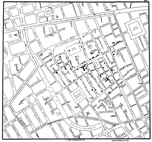
Figure 2. Original map by John Snow showing the clusters of cholera cases in the London epidemic of 1854, drawn and lithographed by Charles Cheffins. Image Public Domain, from Wikipedia.

Snow’s work and dataset can be viewed and thanks to Paul Lindman and others, the work can be expanded: for example, define areas around pumps by walking distance (Fig 3). The R package is cholera. Figure 2 shows a plot like Snow’s annotated map.cholera.
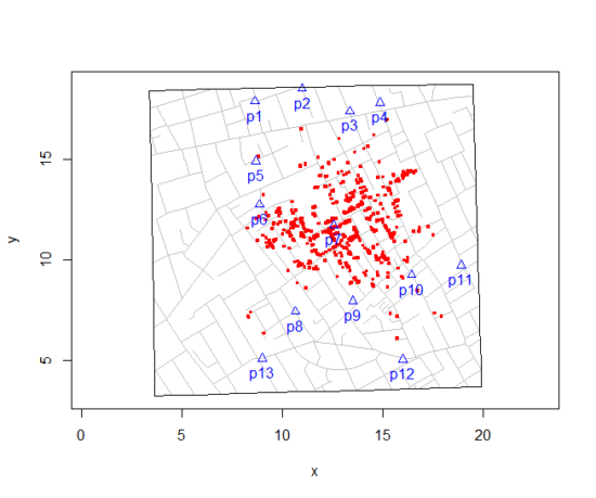
Figure 3. Plot of Snow’s London using R cholera package. Triangles marked with p1-p13 represent public water pumps. Red dots represent cholera cases.
R code to make the plot was
snowMap()Snow’s ideas about cholera were not accepted in his time and you should recognize that by itself, a cluster map supports both the airborne and waterborne theories. The cholera package contains additional data to help visualize the area, including setting regions by walking distance (Fig 4).
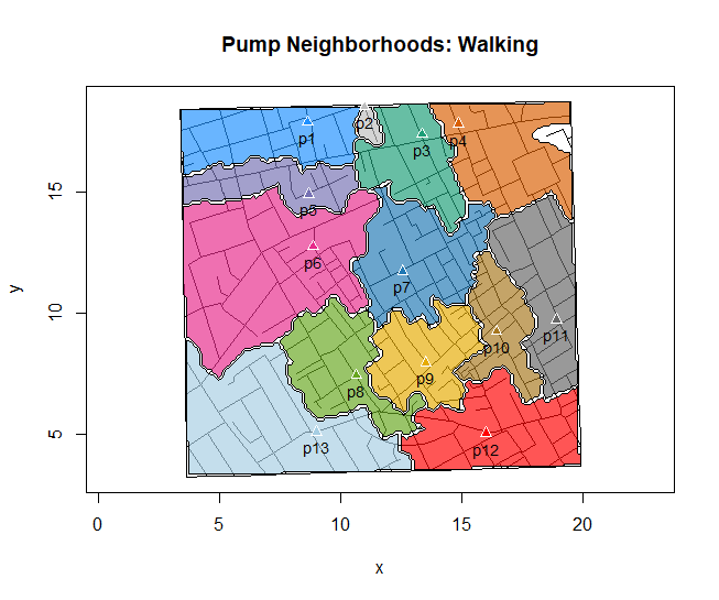
Figure 4. Plot of Snow’s London with walking areas drawn about the 13 water pumps. R cholera package.
R code to make the plot was
plot(neighborhoodWalking(case.set = "expected"), "area.polygons")Epidemiology of cancer.
.
This is an undeveloped section in my book. For now, I’ve listed a number of key landmark studies — a selective and incomplete list — in the history of epidemiology and cancer risk — these would serve well as case studies:
- Tobacco as a carcinogen
- Doll R, Hill AB. Smoking and carcinoma of the lung; preliminary report. Br Med J 1950; 2: 739–748
- Fontham ET, Correa P, Wu-Williams A, Reynolds P, Greenberg RS, Buffler PA, Chen VW, Boyd P, Alterman T, Austin DF, Liff J, Greenberg SD. Lung cancer in non-smoking women: a multicenter case-control study. Cancer Epidemiol Biomarkers Prev 1991;1:35-43
- Diet and cancer risk
- Kolonel LN, Hankin JH, Lee J, Chu SY, Nomura AM, Hinds MW. Nutrient intakes in relation to cancer incidence in Hawaii. Br J Cancer 1981;44:332-339.
- Obesity, exercise, and cancer risk
- Calle EE, Rodriguez C, Walker-Thurmond K, Thun MJ. Overweight, Obesity, and Mortality from Cancer in a Prospectively Studied Cohort of U.S. Adults. N Engl J Med 2003;348:1625-1638.
- Hormones and cancer risk
- Marchbanks PA, McDonald JA, Wilson HG, Folger SG, Mandel MG, Daling JR, Bernstein L, Malone KE, Ursin G, Strom BL, Norman SA, Wingo PA, Burkman RT, Berlin JA, Simon MS, Spirtas R, Weiss LK. Oral contraceptives and the risk of breast cancer. New Engl J Med 2002;346(26):2025-2032.
- Cancer risk and occupations
- absence of cervical cancer but high incidence of breast cancer in nuns (Ramazzini, 1713)
- cancer of the scrotums among chimney sweeps of London (Pott, 1775)
- Silverman DT, Hoover RN, Mason TJ, Swanson GM. Motor exhaust-related occupations and bladder cancer. Cancer Res 1986;46:2113-2116.
Please see review by Greenwald and Dunn (2009).
Questions
- Write up three learning outcomes for this page. Hint: Point your favorite generative AI to this page and ask for help.
- Expand my example of landmark studies (also called pivotal or seminal studies) in epidemiology of cancer to a subject of your own interest. For example, vaccination and communicable diseases like polio.
.
Quiz Chapter 2.3
A history of (bio)statistics
Chapter 2 contents
.
- Introduction
- Why biostatistics?
- Why do we use R Software?
- A brief history of (bio)statistics
- Experimental Design and rise of statistics in medical research
- Scientific method and where statistics fits
- Statistical reasoning
- Chapter 2 – References and suggested reading