20.13 – How to get the distances from a distance tree

Introduction
Example
Molecular clock plot
Questions
References and suggested readings
Chapter 20 contents

Introduction

Extract the patristic distance, the sum of the branch lengths that link two nodes in a tree, for each pair of species.

This distance — see our Chapter 16.6 – Similarity and Distance— is the proportion (p) of amino acid (or nucleotide for DNA or RNA) sites at which the two sequences to be compared are different. It is obtained by dividing the number of amino acid differences by the total number of sites compared. It does not make any correction for multiple substitutions at the same site or differences in evolutionary rates among sites. On a gene tree (Fig. 1), distances are the lengths of the branches connecting the taxa. We want to know how different are two species for the given protein? That’s the distance between them in proportion of amino acid sites that are different by total number compared.

Example

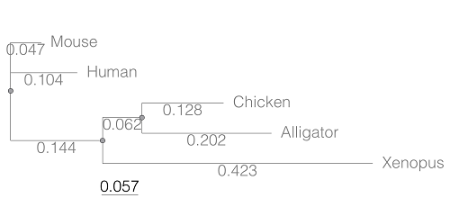
A gene tree of the product (protein HBA1) of five species.

Figure 1. A gene tree of the product (protein HBA1) with five species.

Here’s the Newick format for the tree (HBA1.nwk)

(Mouse:0.0474516,Human:0.104063,((Chicken:0.127652,Alligator:0.202421):0.0616593,Xenopus:0.422801):0.143939);

R code to extract distances and output sorted, pairwise comparisons to a text file

library(ape)

# Create a function
getDis <- function(tree, tips) {
     myTree <- cophenetic(tree)
     myTree <- myTree[,tips]
     xy <- t(combn(colnames(myTree), 2))
     xy <- xy[order(xy[,1], xy[,2]),]
     myOut <- data.frame(xy, myTree[xy])
     colnames(myOut) <- c("Spp1", "Spp2", "Distance")
   return(myOut)
}

# Read a tree file, Newick format
tree5 <-read.tree(text="(Mouse:0.0474516,Human:0.104063,((Chicken:0.127652,Alligator:0.202421):0.0616593,Xenopus:0.422801):0.143939);")

# get taxa names from the tree file
all.tips <- tree5$tip.label; all.tips

# Run the function
myDis <- getDis(tree5, all.tips)

# Check the output
head(myDis)

# Create the results file
write.csv(myDis, file = "my_out.txt")

Example output from head(myDist)

       Spp1    Spp2  Distance
1 Alligator Xenopus 0.6868813
2 Chicken Alligator 0.3300730
3 Chicken   Xenopus 0.6121123
4 Human   Alligator 0.5120823
5 Human     Chicken 0.4373133
6 Human     Xenopus 0.6708030

The function sorts first by Spp1, then by Spp2.

Molecular clock plot

Collect divergence times from timetree.org

Spp1	Spp2	Time (median MYA)
Alligator	Xenopus	352
Chicken	Alligator	245
Chicken	Xenopus	352
Human	Alligator	319
Human	Chicken	319
Human	Xenopus	352

A scatterplot of distance HBA protein sequence by log₁₀-transformed millions of years ago divergence time shown in Figure 2. Note, although tempting, calculating the slope from a linear regression to estimate the rate of evolution would not be appropriate without accounting for the lack of independence of the data (see Phylogenetically independent contrasts). Better methods exist, including calculating rate of change after fitting a model that assumes a strict clock vs relaxed clock.

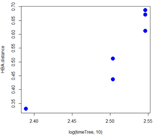
Scatterplot HBA distance by logMYA divergence time

Figure 2. Scatterplot HBA distance by logMYA divergence time

Questions

[pending]

Chapter 20 contents

Additional topics
Area under the curve
Peak detection
Baseline correction
Surveys
Time series
Dimensional analysis
Estimating population size
Diversity indexes
Survival analysis
Growth equations and dose response calculations
Plot a Newick tree
Phylogenetically independent contrasts
How to get the distances from a distance tree
Binary classification
Meta-analysis

/MD

16.4 – Spearman and other correlations

Introduction
Spearman rank correlation
R code
Other correlations
Questions
Quiz
Chapter 16 contents

Introduction

Pearson product moment correlation is used to describe the level of linear association between two variables. There are many types of correlation estimators in addition to the familiar Product Moment Correlation, r.

Spearman rank correlation

If you take the ranks for X₁ and the ranks for X₂, the correlation of ranks is called Spearman rank correlation, r_s. Spearman correlation is a nonparametric statistic. Like the product moment correlation, it can take values between -1 and +1.

For variables X₁ and X₂, the rank order correlation may be calculated on the ranks as

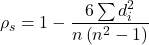
$\begin{align*} \rho_{s} = 1 - \frac{6 \sum d_{i}^2}{n \left (n^2 - 1 \right )} \end{align*}$

where d_i is the difference between the ranks of X₁ and X₂ for each experimental unit. This formula assumes that there are no tied ranks; if there are, use the equation for the product moment correlation instead (but on the ranks).

R commander has an option to calculate the Spearman rank correlation simply by selecting the check box in the correlation sub menu. However, if the data set is small, it may be easier to just run the correlation in the script window.

Our example for the product moment correlation was between Drosophila fly wing length and wing area (Table 1).

Table 1. Fly wing lengths and area, units mm and mm², respectively (Dohm pers obs.)

Obs	Student	Length	Area
1	S01	1.524	0.446
2	S01	2.202	0.876
3	S01	1.52	0.39
4	S01	1.62	0.51
5	S01	1.71	0.736
6	S03	1.551	0.453
7	S03	2.228	0.882
8	S03	1.46	0.394
9	S03	1.659	0.503
10	S03	1.719	0.535
11	S05	1.534	0.441
12	S05	2.223	0.889
13	S05	1.49	0.391
14	S05	1.633	0.514
15	S05	1.704	0.546
16	S08	1.551	0.453
17	S08	2.228	0.882
18	S08	1.468	0.394
19	S08	1.659	0.503
20	S08	1.719	0.535

Repeated observations by image analysis (ImageJ) were collected by four students (S01, S03, So5, S08) from fixed wings to glass slides.

Here’s the scatterplot of the ranks of fly wing length and fly wing area (Fig 1).

fly wings, area by length
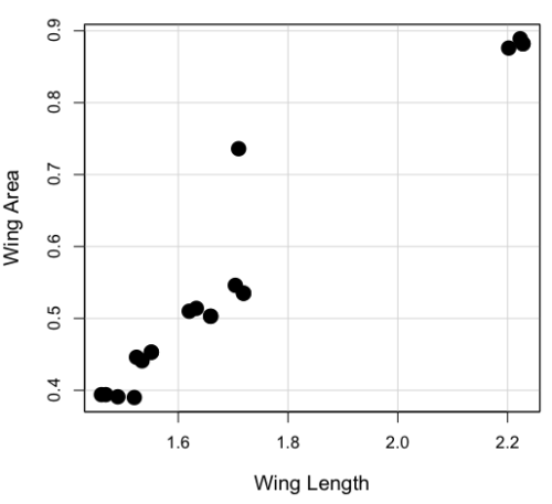
Figure 1. Drosophila wing area (mm²) by wing length (mm).

A nonparametric alternative to the product moment correlation, the Spearman Rank correlation can be obtained directly. The Spearman correlation involves ranking the data, ie, converting data types, from ratio scale data to ordinal scale, then applying the same formula used for the Product moment correlation to the ranked data. The Spearman correlation would be the choice for testing linear association between two ordinal type variables. It is also appropriate in lieu of the parametric product moment correlation when the statistical assumptions are not met, eg, normality assumption.

R code

For the Spearman rank correlation, at the R prompt type

cor.test(Area, Length, alternative="two.sided", method="spearman")

R returns with
    Spearman's rank correlation rho

data:  Area and Length
S = 58.699, p-value = 5.139e-11
alternative hypothesis: true rho is not equal to 0
sample estimates:
      rho 
0.9558658

Alternatively, to calculate either correlation, use R Commander.

Rcmdr: Statistics → Summaries→ Correlation test

Example

BM=c(29,29,29,32,32,35,36,38,38,38,40)
Matings=c(0,2,4,4,2,6,3,3,5,8,6)

cor.test(BM,Matings, method="spearman")
Warning in cor.test.default(BM, Matings, method = "spearman") :
  Cannot compute exact p-value with ties

        Spearman's rank correlation rho

data:  BM and Matings
S = 77.7888, p-value = 0.03163
alternative hypothesis: true rho is not equal to 0
sample estimates:
      rho 
0.6464143

cor.test(BM,Matings, method="pearson")

        Pearson's product-moment correlation

data:  BM and Matings
t = 2.6728, df = 9, p-value = 0.02551
alternative hypothesis: true correlation is not equal to 0
95 percent confidence interval:
 0.1087245 0.9042515
sample estimates:
      cor 
0.6652136

Other correlations

Kendall’s tau

Another nonparametric correlation is Kendall’s tau (τ). Rank the X₁ values, then rank the X₂ values. Count the number of X₁, X₂ pairs that have the same rank (concordant pairs) and the number of X₁, X₂ pairs that do not have the same rank (discordant pairs), Kendall’s tau is then

$\begin{align*} \tau = \frac{\left ( no. \ of \ concordant \ pairs \right ) - \left ( no. \ of \ discordant \ pairs \right ) }{\frac{1}{2} \left ( n - 1 \right )} \end{align*}$

where n is the number of pairs.

Note 1: The denominator is our familiar number of pairwise comparisons if we take k = n

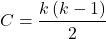
$\begin{align*} C = \frac{k \left ( k - 1 \right )}{2} \end{align*}$

We introduced concordant and discordant pairs when we presented McNemar’s test and cross-classified experimental design in Chapter 9.6.

Example: Judging of Science Fair posters

What is the agreement between two judges, A and B, who evaluated the same science fair posters? Posters were evaluated on if the student’s project was hypothesis-based and judges used a Likert-like scale Strongly disagree (1), Somewhat disagree (2), Neutral (3), Somewhat agree (4), Strongly agree (5).

Table 2. Two judges evaluated six posters for evidence of hypothesis-based project

Poster	Judge.A	Judge.B
1	5	4
2	2	3
3	4	2
4	3	1
5	2	1
6	4	3

A concordant pair represents a poster ranked higher by both judges, while a discordant pair is a poster ranked high by one judge but low by another judge. Poster 1 and poster 5 were concordant pairs,

In R, it is simple to get this correlation directly by invoking the cor.test function and specifying the method equal to kendall. The cor.test assumes that the data are in a matrix, so use the cbind function to bind two vectors together – note the vectors need to have the same number of observations. If the data set is small, it is easier to just enter the data directly in the script window of R commander.

A = c(2,2,3,4,4,5)
B = c(1,3,1,2,3,4)
m = cbind(A,B)
cor.test(A,B, method="kendall")

  Cannot compute exact p-value with ties

        Kendall's rank correlation tau

data:  A and B
z = 1.4113, p-value = 0.1581
alternative hypothesis: true tau is not equal to 0
sample estimates:
      tau 
0.5384615

End of R output

There were no ties in this data set, but we can run the product moment correlation just for comparison

cor.test(A,B, method="pearson")

        Pearson's product-moment correlation

data:  A and B
t = 1.4649, df = 4, p-value = 0.2168
alternative hypothesis: true correlation is not equal to 0
95 percent confidence interval:
 -0.4239715  0.9478976
sample estimates:
      cor 
0.5909091

End R output

Tetrachoric and Polychoric correlation

Tetrachoric correlations used for binomial outcomes (yes, no), polychoric correlation used for ordinal categorical data like the Likert scale. Introduced by Karl Pearson, commonly applied correlation estimate for Item Analysis in psychometric research. Pyschometrics, a sub-discipline within psychology and now a significant part of education research, is about evaluating assessment tools.

R package psych.

R code: Tetrachoric correlation

tetrachoric(x,y=NULL,correct=.5,smooth=TRUE,global=TRUE,weight=NULL,na.rm=TRUE,
     delete=TRUE)

R code: Polychoric correlation

polychoric(x,smooth=TRUE,global=TRUE,polycor=FALSE,ML=FALSE, std.err=FALSE, 
     weight=NULL,correct=.5,progress=TRUE,na.rm=TRUE,  delete=TRUE)

Polyserial correlation

R package polychor. Used to estimate linear association between a ratio scale variable and an ordinal variable.

R code: Polyserial correlation

polyserial(x,y)

Biserial correlation would be a special case of the polyserial correlation, where ordinal variable is replaced by a dichotomous (binomial) variable.

R code: Polyserial correlation

biserial(x,y)

Intra-class correlation coefficient

Both the ICC and the product moment correlation, r, which we introduced in Chapter 16.1, are measures of strength of linear association between two ratio scale variables (Jinyuan et al 2016). But ICC is more appropriate for association between repeat measures of the same thing, eg, repeat measures of running speed. In contrast, the product moment correlation can be used to describe association between any two variables, eg, between repeat measures of running speed, but also between say running speed and maximum jumping height. ICC is used when quantitative measures are organized into paired groups, eg, before and after on same subjects, or cross-classified designs. ICC was introduced in Chapter 12.3 as part of discussion of repeated measures and random effects. ICC is used extensively to assess reliability of a measurement instrument (Shrout and Fleiss 1979; McGraw and Wong 1996).

Example. Data from Table 2

library(psych)
ICC(myJudge, lmer=FALSE)

R output follows

Intraclass correlation coefficients 
                         type  ICC   F df1 df2      p lower bound upper bound
Single_raters_absolute   ICC1 0.40 2.3   5   6  0.166      -0.306        0.84
Single_random_raters     ICC2 0.46 3.9   5   5  0.081      -0.093        0.85
Single_fixed_raters      ICC3 0.59 3.9   5   5  0.081      -0.130        0.90
Average_raters_absolute ICC1k 0.57 2.3   5   6  0.166      -0.880        0.91
Average_random_raters   ICC2k 0.63 3.9   5   5  0.081      -0.205        0.92
Average_fixed_raters    ICC3k 0.74 3.9   5   5  0.081      -0.299        0.95

Number of subjects = 6 Number of Judges = 2
See the help file for a discussion of the other 4 McGraw and Wong estimates

Lots of output, lots of “ICC”. However, rather than explaining each entry, reflect on the type and review the data. Were the posters evaluated repeatedly? Posters were evaluated twice, but only once per judge, so there is a repeated design with respect to the posters. Had the judges been randomly selected from a population of all possible judges? No evidence was provided to suggest this, so judges were a fixed factor (see Chapter 12.3 and Chapter 14.3).

The six ICC estimates reported by R follow discussion in Shrout and Fliess (1979), and our description fits their Case 3: “Each target is rated by each of the same k judges, who are the only judges of interest (p. 421)” Thus, we find ICC for single fixed rater, ICC = 0.59. Note that we would fail to reject the hypothesis that the judges evaluations were associated.

Questions

1. Write up three learning outcomes for this page. Hint: Point your favorite generative AI to this page and ask for help.

2. See Homework 10, Mike’s Workbook for biostatistics

Quiz Chapter 16.4

Spearman and other correlations

Chapter 16 contents

12.1 – The need for ANOVA

Introduction
The multiple comparison problem
Corrections to account for the multiple comparisons problem
ANOVA is a solution
Questions
Quiz
Data used in this page
Chapter 12 contents

Introduction

Moving from an experiment with two groups to multiple groups is deceptively simple: we move from one comparison to multiple comparisons. Consider an experiment in which we have randomly assigned patients to receive one of three doses of a statin drug (lower cholesterol), including a placebo (eg, Tobert and Newman 2015). Thus, we have three groups or levels of a single treatment factor and we’ll want to test the null hypothesis that the group (level) means are all equal as opposed to the alternative hypothesis in which one or more of the group means, eg, group A, Group B, group C, are different.

$\begin{align*} H_{0}: \bar{X}_{A} = \bar{X}_{B} = \bar{X}_{C} \end{align*}$

The correct procedure is to analyze multiple levels of a single treatment with a one-way analysis of variance followed by a suitable post-hoc (“after this”) test. Two common post-hoc tests are Tukey’s range test (aka Tukey’s HSD [honestly significant difference] test), which is for all pairwise comparisons, or the Dunnett’s test, which compares groups against the control group. Post-hoc tests are discussed in Chapter 12.6.

Note. To get the number of pairwise comparisons $C$ of $k$ observations, let

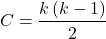
$\begin{align*} C = \frac{k\left ( k-1 \right )}{2} \end{align*}$

for more on pairwise comparisons, see 10.1 – Compare two independent sample means

For our three group experiment, how many pairwise comparisons can be tested? Therefore, $k = 3$ , and we have

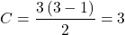
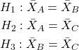
$\begin{align*} C = \frac{3\left ( 3-1 \right )}{2} = 3 \end{align*}$

Thus, for our three groups, A, B, and C, there are three possible pairwise comparisons.

$\begin{align*} H_{1}: \bar{X}_{A} = \bar{X}_{B}\\ H_{2}: \bar{X}_{A} = \bar{X}_{C}\\ H_{3}: \bar{X}_{B} = \bar{X}_{C} \end{align*}$

How many pairwise comparisons for a four group experiment? Check your work, you should get $C = 6$ .

The multiple comparison problem

Let’s say that we’re stubborn. We could do many single two-sample t-tests — certainly, your statistical software won’t stop you — this is a situation that calls for statistical reasoning. Here’s why we should not: we will increase the probability of rejecting a null hypothesis when the null hypothesis is true (eg, discussion in Jafari and Ansari-Pour 2019). That is, the chance we will commit a Type I error increases if we do not account for the lack of independence in these sets of pairwise tests evaluated by t-tests. This is multiplicity or the multiple comparison problem.

Review: when we perform a two-sample t-test we are willing to reject a true null hypothesis 5% of the time. This is what is meant by setting the critical probability value (alpha) = 0.05. By “willing” we mean that we know that our conclusions could be wrong because we ar3 working with samples, not the entire population. (Of course at the time, we have no way of actually knowing WHEN we are wrong, but we do want to know how likely we could be wrong!) However, if we compare three population means we have three separate null hypotheses.

H_O: one or more of the means are different.

But if we conduct these as separate independent sample t-tests, then we are implicitly making the following null hypothesis statements:

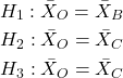
$\begin{align*} H_{1}: \bar{X}_{O} = \bar{X}_{B}\\ H_{2}: \bar{X}_{O} = \bar{X}_{C}\\ H_{3}: \bar{X}_{O} = \bar{X}_{C} \end{align*}$

Thus, we have a 5% chance of being wrong for the first hypothesis and/or a 5% chance of being wrong for the second hypothesis and/or a 5% chance of being wrong for the third hypotheses. The chance that we will be wrong for at least one of these hypotheses must now be greater than 5%.

For three separate hypotheses there is a 14% chance of being wrong when we have the probability value for each individual t-test set at α = 0.05. How did we get this result? The point is that these tests are not independent, they are done on the same data set, therefore you can’t simply apply the multiplication probability rule.

Here’s how to figure this: for the set of three hypotheses, the probability of incorrectly rejecting at least one of the null hypotheses is

$\begin{align*} 1 - 0.953 = 0.14 \end{align*}$

So, for three t-tests on the same experiment, the Type I error overall tests (experiment-wise) is actually 14% not 5%. It gets worse as the number of combinations (groups and therefore hypotheses) increases. For four groups, Type I error is actually

$\begin{align*} 1 - 0.956 = 0.265 \end{align*}$

That’s 26.5%, not 5%.

If we have just five populations means to compare the probability of rejecting a null hypothesis when it is true climbs to 60%! How did this happen? The probability or correctly rejecting all of them is now

$\begin{align*} 0.9510 = 0.599 \end{align*}$

So, the probability of incorrectly rejecting one test (Type I error) is now

$\begin{align*} 1 - 0.9510 = 0.401 \end{align*}$

instead of the 5% we think we are testing.

The key argument for why you must use ANOVA to analyze multiple samples instead of a combination of t-tests!! ANOVA guarantees that the overall error rate is the specified 5%.

Why is the Type I error not 5% for each test? Because we conducted ONE experiment, we can conduct only ONE test (we could be right, we could be wrong 5% of the time). If we conduct the experiment over again, on new subjects, each time resulting in new and therefore independent data sets, then Type I error = 5% for each of these independent experiments.

Now, I hope I have introduced you to the issue of Type I error at the level of a single comparison and the idea of an experiment, holding Type I error-rates at 5% across all hypotheses to be evaluated in an experiment. You may wonder why anyone would make this mistake now. Actually, people make this “mistake” all the time and in some fields like evaluating gene expression for microarray data, this error was the norm, not the exception (see for example discussion of this in Jeanmougin et al 2010).

To conclude, if one does multiple tests on the same experiment, whether it is t-tests or some other test for that matter, then our subsequent tests are related. This is what we mean by independence in statistics — and there are many ways that nonindependence may occur in experimental research. For example, we introduced the concept of pseudoreplication, when observations are treated as if they are independent, but they are not (see Chapter 5.2). The “multiple comparison problem” specifically refers to the lack of independence when all the data set from a single experiment is parsed into lots of separate tests. Philosophically, there must be a logical penalty — and that is reflected in the increase in Type I error.

Clearly something must be done about this!

Corrections to account for the multiple comparisons problem

The family-wise (aka experiment-wise) error rate for multiple comparisons is kept at 5%, and each individual-wise comparison is compared against a more strict (ie, smaller Type I error rate). Put another way, the family-wise error rate is the chance of a number of false positives: making a mistake when we consider many tests simultaneously. The simplest correction for the individual-wise error rate is the Bonferroni correction: test each individual comparison at Type I error equal to $\alpha \slash C$ , where C is the number of comparisons. The Šidák correction, $1-(1-\alpha)^\frac{1}{C}$ , and the Holm-Bonferroni method are alternatives with reportedly better statistical properties (eg, reduced Type II error rates; Ludbrook 1998, Sauder and DeMars 2019).

ANOVA is a solution

One possible solution for getting the correct experiment-wise error rate: adjust for differences in probability for multiple comparisons with the t-test. We used post-hoc tests presented above: you could evaluate the tests after accounting for the change in Type I error. This is what is done in many cases. For example, in genomics. In the early days of gene expression profiling by microarray, it was common to see researchers conduct t-tests for each gene. Since microarrays can have thousands of genes represented on the chip, then these researchers were conducting thousands of t-tests, arranging the t-tests by P-value and counting the number of P-values less than 5% and declaring that the differences were statistically significant.

This error didn’t stand long, and there are now many options available to researchers to handle the “multiple comparisons” problem (some probably better than others, research on this very much an ongoing endeavor in biostatistics). The Bonferroni correction was an available solution, largely replaced by the Holm (aka Holm-Bonferroni) method (Holm 1979). Recall that the Bonferroni correction judged individual p-values statistically significant only if they were less than $\alpha \slash C$ , where, again, α is the family-wise error rate (eg, α = 5%) and C was the number of comparisons. The Holm method orders the C p-values from lowest to highest rank. The method then evaluates lowest p-value, if less than $\alpha \slash C$ , then reject hypothesis for that comparison. Proceed to next p-value, if less than $\alpha \slash C$ , then reject hypothesis for that comparison, and so on until no more comparisons are less than $\alpha \slash C$ .

A MUCH better alternative is to perform a single analysis that takes the multiple-comparisons problem into account: Single Factor ANOVA, also called the one-way ANOVA, plus the post-hoc tests with error correction. We introduce one-way ANOVA in the next section. Post-hoc tests are discussed in Chapter 12.6.

Questions

You should be able to define and distinguish how Bonferoni correction, Dunnett’s test, and Tukey’s test methods protect against inflation of Type I error.
What will be the experiment-wise error rate for an experiment in which there are only two treatment groups?
Experiment-wise error rate may also be called _______________ error rate.
List and compare the three described posthoc approaches to correct for multiple comparison problem,
Glycophosphate-tolerant soybean is the number one GMO (genetically modified organism) crop plant worldwide. Glycophosphate is the chief active ingredient in Roundup, the most widely used herbicide. A recent paper examined “food quality” of the nutrient and elemental composition of plants drawn from fields which grow soy by organic methods (no herbicides or pesticides) and GMO plants subject to herbicides and pesticides. A total of 28 individual t-tests were used to compare the treatment groups for different levels of nutrients and elements (eg, vitamins, amino acids, etc.,); the authors concluded that 10 of these t-tests were statistically significant at Type I error rate of 5%. Discuss the approach to statistical inference by the authors of this report; include correct use of the terms experiment-wise and individual-wise in your response and suggest an alternative testing approach if it is appropriate in your view.
In Chapter 4.2 we introduced a data set from an experiment. The experiment looked at DNA damage quantified by measuring qualities in a Comet Assay including the Tail length, the percent of DNA in the tail, and olive moment. The data set is copied to end of this page. In the next chapter I’ll ask you to conduct the ANOVA on this experiment. For now, answer the following questions.
a. What is the response variable? Defend your choice(s).
b. Why is this an ANOVA problem? Include as part of your explanation a statement of the null hypothesis.

Quiz Chapter 12.1

The need for ANOVA

Data used in this page

comet assay dataset

Treatment	Tail	TailPercent	OliveMoment*
Copper-Hazel	10	9.7732	2.1501
Copper-Hazel	6	4.8381	0.9676
Copper-Hazel	6	3.981	0.836
Copper-Hazel	16	12.0911	2.9019
Copper-Hazel	20	15.3543	3.9921
Copper-Hazel	33	33.5207	10.7266
Copper-Hazel	13	13.0936	2.8806
Copper-Hazel	17	26.8697	4.5679
Copper-Hazel	30	53.8844	10.238
Copper-Hazel	19	14.983	3.7458
Copper	11	10.5293	2.1059
Copper	13	12.5298	2.506
Copper	27	38.7357	6.9724
Copper	10	10.0238	1.9045
Copper	12	12.8428	2.5686
Copper	22	32.9746	5.2759
Copper	14	13.7666	2.6157
Copper	15	18.2663	3.8359
Copper	7	10.2393	1.9455
Copper	29	22.6612	7.9314
Hazel	8	5.6897	1.3086
Hazel	15	23.3931	2.8072
Hazel	5	2.7021	0.5674
Hazel	16	22.519	3.1527
Hazel	3	1.9354	0.271
Hazel	10	5.6947	1.3098
Hazel	2	1.4199	0.2272
Hazel	20	29.9353	4.4903
Hazel	6	3.357	0.6714
Hazel	3	1.2528	0.2506

Data set, comet assay. Rat lung cells treated with Hazel tea extract and exposed to copper metal. Tail refers to length of the comet tail, TailPercent is percent DNA damage in tail, and OliveMoment refers to Olive's (1990), defined as the fraction of DNA in the tail multiplied by tail length

Archive

20.13 – How to get the distances from a distance tree

Introduction

Example

Molecular clock plot

Questions

Suggested readings

Chapter 20 contents

16.4 – Spearman and other correlations

Introduction

Spearman rank correlation

R code

Example

Other correlations

Kendall’s tau

Example: Judging of Science Fair posters

Tetrachoric and Polychoric correlation

R code: Tetrachoric correlation

R code: Polychoric correlation

Polyserial correlation

R code: Polyserial correlation

R code: Polyserial correlation

Intra-class correlation coefficient

Questions

Chapter 16 contents

12.1 – The need for ANOVA

Introduction

The multiple comparison problem

Corrections to account for the multiple comparisons problem

ANOVA is a solution

Questions

Data used in this page

Chapter 12 contents