8.1 – The null and alternative hypotheses
Introduction
Classical statistical parametric tests — t-test (one sample t-test, independent sample-t-test), analysis of variance (ANOVA), correlation, and linear regression— and nonparametric tests like  (chi-square: goodness of fit and contingency table), share several features that we need to understand. It’s natural to see all the details as if they are specific to each test, but there’s a theme that binds all of the classical statistical inference in order to make claim of “statistical significance.”
- a calculated test statistic
- degrees of freedom associated with the calculation of the test statistic
- a probability value or p-value which is associated with the test statistic, assuming a null hypothesis is “true” in the population from which we sample.
- Recall from our previous discussion (Chapter 8.2) that this is not strictly the interpretation of p-value, but a short-hand for how likely the data fit the null hypothesis. P-value alone can’t tell us about “truth.”
- in the event we reject the null hypothesis, we provisionally accept the alternative hypothesis.
Statistical Inference in the NHST Framework
By inference we mean to imply some formal process by which a conclusion is reached from data analysis of outcomes of an experiment. The process at its best leads to conclusions based on evidence. In statistics, evidence comes about from the careful and reasoned application of statistical procedures and the evaluation of probability (Abelson 1995).
Formally, statistics is rich in inference process (Bzdok et al, 2018). We begin by defining the classical frequentist, aka Neyman-Pearson approach, to inference, which involves the pairing of two kinds of statistical hypotheses: the null hypothesis (HO) and the alternative hypothesis (HA). The null hypothesis assumes that any observed difference between the groups are the results of random chance (introduced in Ch 2.3 – A brief history of (bio)statistics ), where “random chance” implies that outcomes occur without order or pattern (Eagle 2021). Whether we reject or accept the null hypothesis — a short-hand for the more appropriate “provisionally reject” in light of the humility that our results may reflect a rare sampling event — based on the outcome of our statistical inference, the inference is evaluated against a decision criterion (cf discussion in Christiansen 2005), a fixed statistical significance level (Lehmann 1992). Significance level refers to the setting of a p-value threshold before testing is done. The threshold is often set to Type I error of 5% (Cowles & Davis 1982), but researchers should always consider whether this threshold is appropriate for their work (Benjamin et al 2017).
This inference process is referred to as Null Hypothesis Significance Testing, NHST. Additionally, a probability value will be obtained for the test outcome or test statistic value. In the Fisherian likelihood tradition, the magnitude of this statistic value can be associated with a probability value, the p-value, of how likely the result is given the null hypothesis is “true.” (Again, keep in mind that this is not strictly the interpretation of p-value, it’s a short-hand for how likely the data fit the null hypothesis. P-value alone can’t tell us about “truth”, per our discussion, Chapter 8.2.)
Note 1: About reporting p-values, -logP. A Google search will likely reveal “logP,” which is a measure in chemistry. In contrast, “-logP” pertains to how to report p-values in statistics. P-values are traditionally reported as a decimal, like 0.000134, in the closed (set) interval (0,1) — p-values can never be exactly zero or one. The smaller the value, the less the chance our data agree with the null prediction. Small numbers like this can be confusing, particularly if many p-values are reported, like in many genomics works, eg, GWAS studies. In the past, small p-values would be reported as “less than,” eg, < 0.001. This was done in part because of the misleading impression of precision that many significant figures can represent (see discussion in Lang and Altman 2014).
-logP is an alternative, particularly for GWAS studies where the significance level may be much smaller than 5%. Thus, instead of reporting vanishingly small p-values, studies may report the negative log10 p-value, or -logP. Instead of small numbers, large numbers are reported, the larger, the more against the null hypothesis. Thus, our p-value becomes 3.87 -logP.
R code
-1*log(0.000134,10)
[1] 3.872895
Why log10 and not some other base transform? Just that log10 is convenience — powers of 10.
The antilog of 3.87 returns our p-value
> 10^(-1*3.872895)
[1] 0.0001340001
For convenience, a partial p-value -logP transform table
| P-value | -logP |
| 0.1 | 1 |
| 0.01 | 2 |
| 0.001 | 3 |
| 0.0001 | 4 |
On your own, complete the table up to -logP 5 – 10. See Question 7 below.
NHST Workflow
We presented in the introduction to Chapter 8 without discussion a simple flow chart to illustrate the process of decision (Fig 1, Chapter 8). Here, we repeat the flow chart diagram and follow with descriptions of the elements.
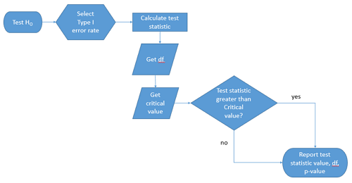
Figure 1. Flow chart of inductive statistical reasoning.
What’s missing from the flow chart is the very necessary caveat that interpretation of the null hypothesis is associated with two kinds of error, Type I error and Type II error. These points and others are discussed in the following sections.
We start with the hypothesis statements. For illustration we discuss hypotheses in terms of comparisons involving just two groups, also called two sample tests. One sample tests in contrast refer to scenarios where you compare a sample statistic to a population value. Extending these concepts to more than two samples is straightforward, but we leave that discussion to Chapters 12 – 18.
Null hypothesis
By far the most common application of the null hypothesis testing paradigm involves the comparisons of different treatment groups on some outcome variable. These kinds of null hypotheses are the subject of Chapters 8 through 12.
The Null hypothesis (HO) is a statement about the comparisons, eg, between a sample statistic and the population, or between two treatment groups. The former is referred to as a one tailed test whereas the latter is called a two-tailed test. The null hypothesis is typically “no statistical difference” between the comparisons.
For example, a one sample, two tailed null hypothesis.

and we read it as “there is no statistical difference between our sample mean and the population mean.” For the more likely case in which no population mean is available, we provide another example, a two sample, two tailed null hypothesis.

Here, we read the statement as “there is no difference between our two sample means.” Equivalently, we interpret the statement as both sample means estimate the same population mean.

Under the Neyman-Pearson approach to inference we have two hypotheses: the null hypothesis and the alternative hypothesis. The hull hypothesis was defined above.
Note 2: Tails of a test are discussed further in chapter 8.4.
Alternative hypothesis
Alternative hypothesis (HA): If we conclude that the null hypothesis is false, or rather and more precisely, we find that we provisionally fail to reject the null hypothesis, then we provisionally accept the alternative hypothesis. The view then is that something other than random chance has influenced the sample observations. Note that the pairing of null and alternative hypotheses covers all possible outcomes. We do not, however, say that we have evidence for the alternative hypothesis under this statistical regimen (Abelson 1995). We tested the null hypothesis, not the alternative hypothesis. Thus, it is incorrect to write that, having found a statistical difference between two drug treatments, say aspirin and acetaminophen for relief of migraine symptoms, it is not correct to conclude that we have proven the case that acetaminophen improves improves symptoms of migraine sufferers.
For the one sample, two tailed null hypothesis, the alternative hypothesis is

and we read it as “there is a statistical difference between our sample mean and the population mean.” For the two sample, two tailed null hypothesis, the alternative hypothesis would be

and we read it as “there is a statistical difference between our two sample means.”
Alternative hypothesis often may be the research hypothesis.
It may be helpful to distinguish between technical hypotheses, scientific hypothesis, or the equality of different kinds of treatments. Tests of technical hypotheses include the testing of statistical assumptions like normality assumption (see Chapter 13.3) and homogeneity of variances (Chapter 13.4). The results of inferences about technical hypotheses are used by the statistician to justify selection of parametric statistical tests (Chapter 13). The testing of some scientific hypothesis like whether or not there is a positive link between lifespan and insulin-like growth factor levels in humans (Fontana et al 2008), like the link between lifespan and IGFs in other organisms (Holtzenberger et al 2003), can be further advanced by considering multiple hypotheses and a test of nested hypotheses and evaluated either in Bayesian or likelihood approaches (Chapter 16 and Chapter 17). The advantage of the Bayesian approach is that it returns evidence for or against this hypothesis: if the posterior probability is greater than the prior probability, we can we say that we have evidence for the hypothesis. This is very appealing — the challenge is that the prior probability is inherently subjective (Chapter 6.4), limited by the amount and quality of existing information pertaining to the hypothesis (Prelec 2004).
Note 3: In Bayesian statistics, hypotheses and their parameters are treated as random variables and we can assign them probabilities. The prior probability is your initial belief about the likelihood of an event before adding new data. The posterior probability is the updated probability after new data has been added. Thus, the posterior combines your prior belief with the new information (the likelihood).
In the frequentis approach, the null hypothesis is no difference (no effect); in the Bayesian context, we’d treat this as a point estimate of zero and have to assign it a probability. In the absence of empirical evidence, one option is to set the probability as 50%, equal prior odds. Use of the spike and slab prior is likely a better approach. There’s a lot of work on these points; I refer interested readers to Campbell and Gustafson (2024) for additional readings and discussion.
How to interpret the results of a statistical test.
Any number of statistical tests may be used to calculate the value of the test statistic. For example, a one sample t-test may be used to evaluate the difference between the sample mean and the population mean (Chapter 8.5) or the independent sample t-test may be used to evaluate the difference between means of the control group and the treatment group (Chapter 10). The test statistic is the particular value of the outcome of our evaluation of the hypothesis and it is associated with the p-value. In other words, given the assumption of a particular probability distribution, in this case the t-distribution, we can associate a probability, the p-value, that we observed the particular value of the test statistic and the null hypothesis is true in the reference population.
By convention, we determine statistical significance (Cox 1982; Whitley & Ball 2002) by assigning ahead of time a decision probability called the Type I error rate, often given the symbol α (alpha). The practice is to look up the critical value that corresponds to the outcome of the test with degrees of freedom like your experiment and at the Type I error rate that you selected. The Degrees of Freedom (DF, df, or sometimes noted by the symbol v), are the number of independent pieces of information available to you. Knowing the degrees of freedom is a crucial piece of information for making the correct tests. Each statistical test has a specific formula for obtaining the independent information available for the statistical test. We first were introduced to DF when we calculated the sample variance with the Bessel correction, n – 1, instead of dividing through by n. With the df in hand, the value of the test statistic is compared to the critical value for our null hypothesis. If the test statistic is smaller than the critical value, we fail to reject the null hypothesis. If, however, the test statistic is greater than the critical value, then we provisionally reject the null hypothesis. This critical value comes from a probability distribution appropriate for the kind of sampling and properties of the measurement we are using. In other words, the rejection criterion for the null hypothesis is set to a critical value, which corresponds to a known probability, the Type I error rate.
Before proceeding with yet another interpretation, and hopefully less technical discussion about test statistics and critical values, we need to discuss the two types of statistical errors. The Type I error rate is the statistical error assigned to the probability that we may reject a null hypothesis as a result of our evaluation of our data when in fact in the reference population, the null hypothesis is, in fact, true. In Biology we generally use Type I error α = 0.05 level of significance. We say that the probability of obtaining the observed value AND HO is true is 1 in 20 (5%) if α = 0.05. Put another way, we are willing to reject the Null Hypothesis when there is only a 5% chance that the observations could occur and the Null hypothesis is still true. Our test statistic is associated with the p-value; the critical value is associated with the Type I error rate. If and only if the test statistic value equals the critical value will the p-value equal the Type I error rate.
The second error type associated with hypothesis testing is, β, the Type II statistical error rate. This is the case where we accept or fail to reject a null hypothesis based on our data, but in the reference population, the situation is that indeed, the null hypothesis is actually false. We must also keep in mind that, as we evaluate the p-value relative to the magnitude of the Type I error rate, and if we reject the null hypothesis, we still do not say that we have evidence for the alternative hypothesis.
Thus, we end with a concept that may take you a while to come to terms with — there are four, not two possible outcomes of an experiment.
Outcomes of an experiment
What are the possible outcomes of a comparative experiment\? We have two treatments, one in which subjects are given a treatment and the other, subjects receive a placebo. Subjects are followed and an outcome is measured. We calculate the descriptive statistics aka summary statistics, means, standard deviations, and perhaps other statistics, and then ask whether there is a difference between the statistics for the groups. So, two possible outcomes of the experiment, correct\? If the treatment has no effect, then we would expect the two groups to have roughly the same values for means, etc., in other words, any difference between the groups is due to chance fluctuations in the measurements and not because of any systematic effect due to the treatment received. Conversely, then if there is a difference due to the treatment, we expect to see a large enough difference in the statistics so that we would notice the systematic effect due to the treatment.
Actually, there are four, not two, possible outcomes of an experiment, just as there were four and not two conclusions about the results of a clinical assay. The four possible outcomes of a test of a statistical null hypothesis are illustrated in Table 1.
Table 1. When conducting hypothesis testing, four outcomes are possible.
| HO in the population | |||
| True | False | ||
| Result of statistical test | Reject HO | Type I error with probability equal to
α (alpha) |
Correct decision, with probability equal to
1 – β (1 – beta) |
| Fail to reject the HO | Correct decision with probability equal to
1 – α (1 – alpha) |
Type II error with probability equal to
β (beta) |
|
In the actual population, a thing happens or it doesn’t. The null hypothesis is either true or it is not. But we don’t have access to the reference population, we don’t have a census. In other words, there is truth, but we don’t have access to the truth. We can weight, assigned as a probability or p-value, our decisions by how likely our results are given the assumption that the truth is indeed “no difference.”
If you recall, we’ve seen a table like Table 1 before in our discussion of conditional probability and risk analysis (Chapter 7.3). We made the point that statistical inference and the interpretation of clinical tests are similar (Browner and Newman 1987). From the perspective of ordering a diagnostic test, the proper null hypothesis would be the patient does not have the disease. For your review, here’s that table (Table 2).
Table 2. Interpretations of results of a diagnostic or clinical test.
| Does the person have the disease\? | |||
| Yes | No | ||
| Result of the diagnostic test |
Positive | sensitivity of the test (a) | False positive (b) |
| Negative | False negative (c) | specificity of the test (d) | |
Thus, a positive diagnostic test result is interpreted as rejecting the null hypothesis. If the person actually does not have the disease, then the positive diagnostic test is a false positive.
Questions
- Match the corresponding entries in the two tables. For example, which outcome from the inference/hypothesis table matches specificity of the test \?
- Find three sources on the web for definitions of the p-value. Write out these definitions in your notes and compare them.
- In your own words distinguish between the test statistic and the critical value.
- All of our discussions have been about testing the null hypothesis, about accepting or rejecting, provisionally, the null hypothesis.
- What are the p-values for -logP of 5, 6, 7, 8, 9, and 10 \? Complete the p-value -logP transform table.
- Instead of log10 transform, create a similar table but for negative natural log transform. Which is more convenient? Hint:
log(x, base=exp(1))
Quiz Chapter 8.1
The null and alternate hypothesis
Chapter 8 contents
8 – Inferential statistics
Introduction
Statistical methods are important in biology because results of experiments are usually not clear-cut and therefore tests to support decisions between competing hypotheses are needed.
We will limit ourselves to a general discussion with examples, but beginning in this chapter, we start our introductions of specific types of statistical tests. As a reminder, our statistical philosophy is frequentist and follows the Null Hypothesis Significance Testing or NHST approach. Discussion of Bayesian statistical approaches are included as appropriate.
Thus, all statistical tests we will talk about share the following requirements or properties.
- The type of data we have dictates which test or tests are appropriate.
- We start with a clear description of the null hypotheses.
- (Fig 1, Test H0). See Chapter 8.1.
- Set the Type I error rate, alpha, α (Fig 1, Select Type I error rate).
- By convention, 5% is often used (Cowles and David 1982).
- See also our discussion in Chapter 8.1 and Chapter 8.2.
- We must be aware of the assumptions our statistical tests make and what, if any, modifications to them we can make.
- Assumptions of parametric tests are discussed in Chapter 13.
- Correct computation of the test statistic and degrees of freedom.
- Fig 1, Calculate test statistics and get df.
- Each statistical test results in a test statistic with associated degrees of freedom. These are described in chapters and chapter sections devoted to the different kinds of statistical tests.
- Comparison of the critical value and the test statistic value, with interpretation and significance testing (p-value, Bayesian Factor, cf. discussion in Goodman 2008).
- Fig 1, Test statistic greater than critical value?
- Report result: Fig 1, test statistic value, df, and p-value.
- Interpretation of p-value is done throughout the rest of this book, but in earnest, discussion is presented in Chapter 8.2.
We can provide a flow-chart of these steps (Fig 1).
Figure 1. NHST decision flow chart.
While we want to avoid the impression that statistical analysis is simply a matter of following a step-by-step protocol (Fig 1), it nevertheless may be helpful to think of it as such, understanding all the while that there are caveats and assumptions that accompany the choices we make while following the protocol.
Suggested homework
Quizzes in this chapter
A total of 38 questions among the several subchapters, a mix of true or false and multiple choice question format.
Chapter 8 contents
6.9 – Chi-square distribution
Introduction
As noted earlier, the normal deviate or Z score can be viewed as randomly sampled from the standard normal distribution. The chi-square distribution describes the probability distribution of the squared standardized normal deviates with degrees of freedom, df, equal to the number of samples taken. (The number of independent pieces of information needed to calculate the estimate, see Ch. 8.) We will use the chi-square distribution to test statistical significance of categorical variables in goodness of fit tests and contingency table problems.
The equation of the chi-square is
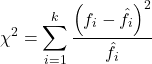
where k is the number of groups or categories, from 1 to k, and fi is the observed frequency and fi “hat” is the expected frequency for the kth category. We call the result of this calculation the chi-square test statistic. We evaluate how often that value or greater of a test statistic will occur by applying the chi-square distribution function. Graphs to show chi-square distribution for degrees of freedom equal to 1 – 5, 10, and 20 (Fig 1).
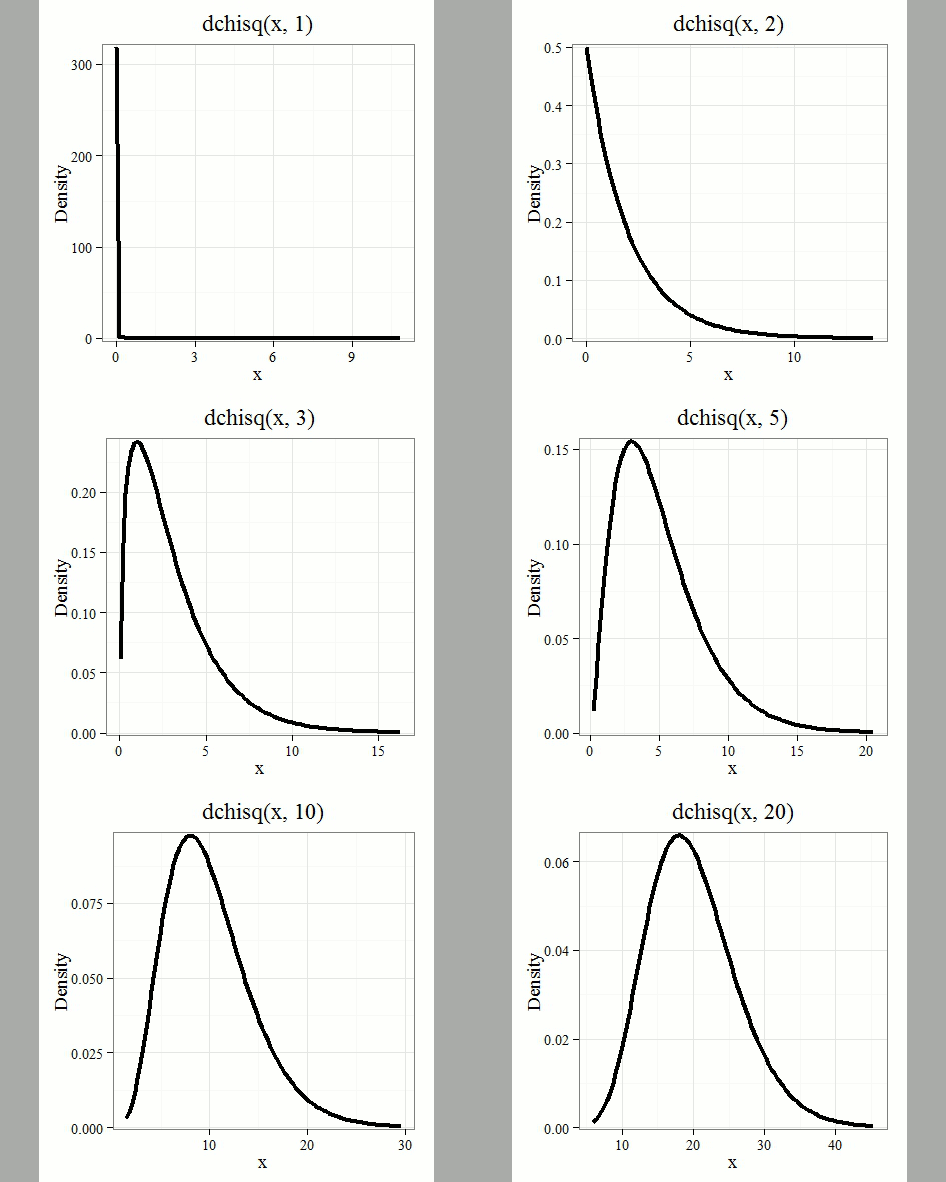
Figure 1. Animated GIF of plots of chi-square distribution over range of degrees of freedom.
Note that the distribution is asymmetric, particularly at low degrees of freedom. Thus tests using the chi-square are one-tailed (Fig 2).
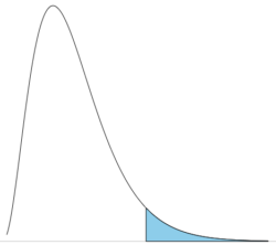
Figure 2. The test of the chi-square is typically one-tailed. In this case, probability of values greater than the critical value.
By convention in the Null Hypothesis Significance Testing protocol (NHST), we compare the test statistic to a critical value. The critical value is defined as the value of the test statistic — the cutoff boundary between statistical significance and insignificance — that occurs at the Type I error rate, which is typically set to 5%. The interpretation of the result is as follows: after calculating a test statistic, we can judge significance of the results relative to the null hypothesis expectation. If our test statistics is greater than the critical value, then the p-value of our results are less than 5% (R will report an exact p-value for the test statistic). You are not expected to be able to follow this logic just yet — rather, we teach it now as a sort of mechanical understanding to develop in the NHST tradition. The justification for this approach to testing of statistical significance is developed in Chapter 8. A portion of the critical values of the chi-square distribution are shown in Figure 3.
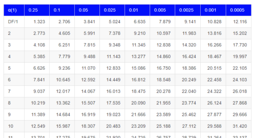
Figure 3. Portion of the table of some critical values of chi-square distribution, one tailed (right-tailed or “upper” portion of distribution).
See Appendix for a complete chi-square table.
The chi-squared test is a one-tailed test.
The result of the calculation of the test statistic is always non-negative because it is calculated by squaring the differences between the observed and expected frequencies. As a consequence, the test is always “right-tailed.”
The chi-square test does not provide information about the direction of an association, nor the strength of the association, only whether or not the variables are independent or associated. We use “correlation,” (eg, Phi coefficient or Cramer’s V, see Chapter 9.1 – Chi-square test: Goodness of fit and Chapter 9.2 – Chi-square contingency tables), to quantify the strength and direction of the association. While statistical significance is important, examining the direction and magnitude, the effect size, provides actionable insight and context for making informed decisions. For example, a new drug tested in a clinical trial may show an association between subject improvement (statistical significance), but yet have a small effect.
Example
Professor Hermon Bumpus of Brown University in Providence, Rhode Island, received 136 House Sparrows (Passer domesticus) after a severe winter storm 1 February 1898. The birds were collected from the ground; 72 of the birds survived, 64 did not (Table 1). Bumpus made several measures of morphology on the birds and the data set has served as a classical example of Natural Selection (Chicago Field Museum). We’ll look at this data set when we introduce Linear Regression.
Table 1. Survival statistics of Bumpus House sparrows
| Yes | No | |
| Female | 21 | 28 |
| Male | 51 | 36 |
Was there a survival difference between male and female House Sparrows? This is a classic contingency table analysis, something we will at length in Chapter 9. For now, we report the Chi-square test statistic for this test was 3.1264 and the test had one degree of freedom. What is the critical value of the chi-square distribution at 5% and one degree of freedom?. Typically we would simply use R to look this up
qchisq(c(0.05), df=1, lower.tail=FALSE)
But we can also get this from the table of critical values (Fig 4). Simply select the row based on the degrees of freedom for the test then scan to the column with the appropriate significance level, again, typically 5% (0.05).
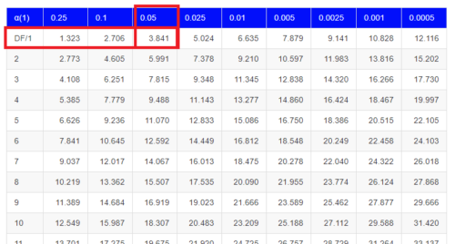
Figure 4. Portion of the chi-square distribution which shows how to find critical value of the chi-square distribution.
For 1 degree of freedom at 5% significance, the critical value is 3.841. Back to our hypothesis: Did male and female survival differ in the Bumpus data set? Following the NHST logic, if the test statistic value (eg, 3.1264) is greater than the critical value (3.841), then we would reject the null hypothesis. For this example, we would conclude no statistical difference between male and female survival because the test statistic was smaller than the critical value. How likely are these results due to chance? That’s where the p-value comes in. Our test statistic value falls between 5% and 10% (2.706 < 3.1264 < 3.841). In order to get the actual p-value of our test statistic we would need to use R.
R code
Given a chi-square test statistic you can use R to calculate the probability of that value against the null hypothesis. At the R prompt
pchisq(c(3.1264), df=1, lower.tail=FALSE)
And R output
[1] 0.07703368
Because we are using R Commander, simply select the command by following the menu options.
Rcmdr: Distributions → Continuous distributions → Chi-squared distribution → Chi-squared probabilities …
Enter the chi-square value and degrees of freedom (Fig 5).
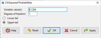
Figure 5. Screenshot of input box in Rcmdr for Chi-square probability values.
Questions
- What happens to the shape of the chi-square distribution as degrees of freedom are increased from 1 to 5 to 20 to 100?
Be able to answer these questions using the Chi-square table, Appendix 20.2, or using Rcmdr
- For probability α = 5%, what is the critical value of the chi-square distribution (upper tail)?
- The value of the chi-square test statistic is given as 12. With 3 degrees of freedom, what is the approximate probability of this value, or greater from the chi-square distribution?
Quiz Chapter 6.9
Chi-square distribution
Chapter 6 contents
- Introduction
- Some preliminaries
- Ratios and proportions
- Combinations and permutations
- Types of probability
- Discrete probability distributions
- Continuous distributions
- Normal distribution and the normal deviate (Z)
- Moments
- Chi-square (Χ2) distribution
- t distribution
- F distribution
- References and suggested readings
4 – How to report statistics
Introduction: Reporting your results.
While you are thinking about exploring data sets and descriptive statistics, please review our overview of data analysis (Chapter 2.4 and 2.5). While the scientific hypotheses come first, how experiments are designed should allow for straight-forward analysis: in other words, statistics can’t rescue poorly designed experiments, nor can it reveal new insight after the fact.
Once the experiments are completed, all projects will go through a similar process:
- Description: Describe and summarize the results.
- Check assumptions.
- Inference: conduct tests of hypotheses.
- Develop and evaluate statistical models.
Clearly this is a simplification, but there’s an expectation your readers will have about a project. Basic questions like how many subjects got better on the treatment? Is there an association between Body Mass Index (BMI) and the primary outcome? Did male and female subjects differ for response to the treatment? Undoubtedly these and related questions form the essence of the inferences, but providing graphs to show patterns may be as important to a reader as any p-value — a number which describes how likely it is that your data would have occurred by chance — eg, from an Analysis of variance.
Each project is unique — sorry, what a breathtakingly obvious statement — but what elements must be included in a results section?
Data visualization.
We describe data in three ways: graphs, tables, and in sentences. In this page we present the basics of when to choose a graph over presenting data in a table or as a series of sentences (ie, text). In the rest of this chapter we introduce the various graphics we will encounter in the course. Chapter 4 covers eight different graphics, but is by no means an exhaustive list of kinds of graphs. Phylogenetic network graphs are presented in Chapter 20.11. Although an important element of presentation in journal articles, we don’t discuss figure legends or table titles; guidelines are typically available by the journal of choice (eg, PLOS ONE journals guidelines).
A quick note about terminology. Data visualization encompasses charts, graphs and plots. Of the three terms, chart is the more generic. Graphs are used to display a function or mapping between two variables; plots are kinds of graphs for a finite set of points. There is a difference among the terms, but I confess, I won’t be consistent. Instead, I will refer to each type of data visualization by its descriptive name: bar chart, box plots, histograms, scatter plot, etc. Note that technically, a scatter plot can refer to a graph, eg, a line drawn to reflect a linear association between the two variables, whereas bar charts and box plots would not be a graph because no function is implied.
Why display data?
Do we just to show a graph to break the monotony of page after page of text or do we attempt to do more with graphs? After all, isn’t “a picture’s worth a thousand words?” In many cases, yes! Graphics allow us to see patterns. Data visualization is a key part of exploratory data analysis (Tukey 1977), or data mining in the parlance of big data (Keim 2001). Data visualization is also a crucial tool in the public health arena, and finding effective graphics to communicate, at times, complex data and information to both public and professional audiences can be challenging (see discussion in Meloncon and Warner 2017).
Graphics are complicated — all the interplay among pixels etc and rendering process — and expensive to do well. Text is much cheaper to publish, even in digital form. But the ability to visualize concepts, that is, to connect ideas to data through our eyes (see Wikipedia), seems to be more the cognitive goal of graphics. Lofty purpose, desirable goal. Yes, it is true that graphics can communicate concepts to the reader, but with some caution. Images distort, and default options in graphics programs are seldom acceptable for conveying messages without bias (Glazer 2011).
Here’s some tips from a book on graphical display (Tufte 1983; see also Camões 2016).
Your goal is to communicate complex ideas with clarity, precision, and efficiency. Graphical displays should:
- show the data
- avoid distorting the data
- present numbers in a small space
- help the viewer’s eye to compare different pieces of data
- serve a clear purpose (description, exploration, tabulation, decoration)
- be closely integrated with statistical and verbal descriptions of a data set.
We accomplish these tasks by following general principles involving scale and a commitment to avoiding bias in our presentation.
Importantly, graphs can show patterns not immediately evident in tables of numbers. See Table 1 for an example of a dataset, “Anscombe’s quartet,” (Anscombe 1973), where a picture is clearly helpful.
Anscombe’s quartet
| X | Y1 | Y2 | Y3 | Y4 |
|---|---|---|---|---|
| 10 | 8.04 | 9.14 | 7.46 | 6.58 |
| 8 | 6.95 | 8.14 | 6.77 | 5.76 |
| 13 | 7.58 | 8.74 | 12.74 | 7.71 |
| 9 | 8.81 | 8.77 | 7.11 | 8.84 |
| 11 | 8.33 | 9.26 | 7.81 | 8.47 |
| 14 | 9.96 | 8.10 | 8.84 | 7.04 |
| 6 | 7.24 | 6.13 | 6.08 | 5.25 |
| 4 | 4.26 | 3.10 | 5.39 | 12.50 |
| 12 | 10.84 | 9.13 | 8.15 | 5.56 |
| 7 | 4.82 | 7.26 | 6.42 | 7.91 |
| 5 | 5.68 | 4.74 | 5.73 | 6.89 |
| Mean (±SD) | 7.50 (2.032) | 7.50 (2.032) | 7.50 (2.032) | 7.50 (2.032) |
The Anscombe dataset is also available in R packages data(Anscombe, package="carData"), or you can copy/paste from Table 1 into a spreadsheet or text file, then load the data file into R (eg, Rcmdr → Load data set). Note that the data set does not include the column summary statistics shown in the last row of the table.
Before proceeding, look again at the table — See any patterns in the table?
Maybe.… Need to be careful as we humans are really good at perceiving patterns, even when no pattern exists.
Now, look just at the last row in the table, the row containing the descriptive statistics (the means and standard deviations). Any patterns?
The means and standard deviations are the same, so nothing really jumps out at you — does that mean that there are no differences among the columns then?
But let’s see what the scatter plots look like before we conclude that the columns of Y ’s are the same (Fig. 1). I’ll also introduce the R package clipr, which is useful for working with your computer’s clipboard.
Note 1: To show clipboard history, on Windows press + V; on macOS, open Finder and select Edit → Show Clipboard.
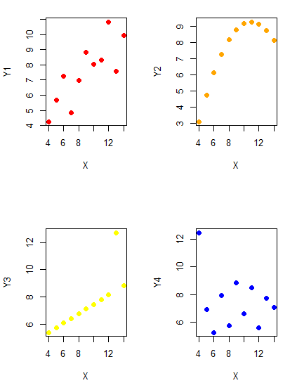
Figure 1. Scatter plot graphs of Anscombe’s quartet (Table 1)
#R code for Figure 1.

require(clipr)
#Copy from the Table and paste into spreadsheet (exclude last row). Highlight and copy data in spreadsheet
myTemp <- read_clip_tbl(read_clip(), header=TRUE, sep = "\t")
#Check that the data have been loaded correctly
head(myTemp)
#attach the data frame, so don't have to refer to variables as myTemp\$variable name
attach(myTemp)
#set the plot area for 4 graphs in 2X2 frame
par(mfrow=c(2,2))
plot(X, Y1, pch=19, col="red", cex=1.2)
plot(X, Y2, pch=19, col="orange",cex=1.2)
plot(X, Y3, pch=19, col="yellow",cex=1.2)
plot(X, Y4, pch=19, col="blue",cex=1.2)
And now we can see that the Y ‘s have different stories to tell. While the summary (descriptive) statistics are the same, the patterns of the association between Y values and the X variable are qualitatively different: Y1 is linear, but diffuse; Y2 is nonlinearly associated with X; Y3, like Y1, is linearly related to X, but one data point seems to be an outlier; and for Y4 we see a diffuse nonlinear trend and an outlier.
So, that’s the big picture here. In working with data, you must look at both ways to “see” data — you need to make graphs and you also need to calculate basic descriptive statistics.
And as to the reporting of these results, sometimes Tables are best (i.e., so others can try different statistical tests), but patterns can be quickly displayed with carefully designed graphs. Clearly, in this case, the graphs were very helpful to reveal trends in the data.
When to report numbers in a sentence? In a table? In a graph?
The choice depends on the message. Usually you want to make a comparison (or series of comparisons). If you are reporting one or two numbers in a comparison, a sentence is fine. “The two feral goat populations had similar mean numbers (120 vs. 125) of kids each breeding period.” If you have only a few comparisons to make, the text table is useful:
Table 2. Data from Kipahoehoe Natural Area Reserve, SW slope of Mauna Loa.
| Location | Number of kids |
|---|---|
| Outside fence | |
| kīpuka | 51 |
| other | 120 |
| Inside fence | |
| kīpuka | 3 |
To conclude, tables are the best way to show exact numbers and tables are preferred over graphs when many comparisons need to be made.
Note 2: A kīpuka is a land area surrounded by recent lava flows. This was a real data set, but I’ve misplaced the citation!
Couldn’t I use a pie chart for this?
Yes, but I will try and persuade you to not. Pie charts are used to show part-whole relationships. If there are just a few groups, and if we don’t care about precise comparisons, pie charts may be effective. Some good examples are Figure 1 O’Neill et al 2020,
Sometimes, people use pie charts for very small data sets (comparing two populations, or three categories, for example). These work well, but as we increase the number of categories, the graphic likely requires additional labels and remarks to clarify the message. The problem with pie charts is that they require interpretation of the angles that define the wedges, so we can’t be very precise about that. Bar charts are much better than pie charts — but can also suffer when many categories are used (Chapter 4.1).
To illustrate the problem, here’s a couple of pie charts from Microsoft Excel (a similar chart can be made with LibreOffice Calc) for our goat data set; compare this graph to the table and to the bar chart below (Fig 2).
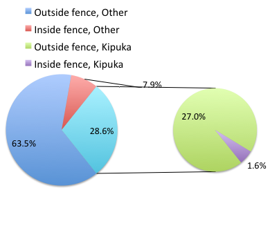
Figure 2. Excel pie chart of Table 2 data set.
A bar chart of the same data (Fig 3).
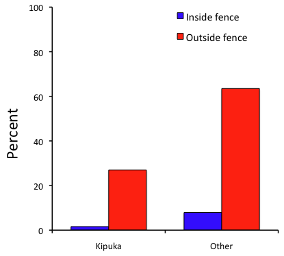
Figure 3. Bar chart of Table 2 data set
The bar chart (Fig 3) is easier to get the message across; more goat kids were found outside the fenced area then inside the fenced in areas. We can also see that more goat kids were found in the “other” areas compared to the kipuka. The pie chart (Fig 2) in my opinion fails to communicate these simple comparisons, conclusions about patterns in the data that clearly would be the take-home message from this project. Aesthetically the bar chart could be improved — a mosaic plot would work well to show the associations in the project results (See Ch 4.4 Mosaic plots). Furthermore, a strong case can be made that the bar chart is over kill — after all, there’s only the four points to show.
Note 3: A much better graph would include the actual counts, eg, a box plot as discussed in Chapter 4.3.
But we are not done with this argument, to use graphics or text to report results. Neither the bar chart (mosaic plot) or the pie chart really work. The reader has to interpret the graphics by extrapolating to the axes to get the numbers. While it may be boring — 1.5 million hits Google search “data tables” boring — tables can be used for comparisons and make the patterns more clear and informative to the reader. Here’s a different version of the table to emphasize the influence of fencing on the goat population.
Table 3. Revised Table 2 to emphasize comparisons between inside and outside the fence line on feral goat population on Mauna Loa.
| Location | Kīpuka | Other |
|---|---|---|
| Outside fence | 51 | 120 |
| Inside fence | 3 | 15 |
Table 3 would be my choice — over a sentence and over a graph. At a glance I can see that more goat kids were found outside of the fenced area, regardless of whether it was in a kipuka or some other area on the mountain side. Table 3 is an improvement over Table 2 because it presents the comparisons in a 2 X 2 format — especially useful when we have a conditional set.
For example, it’s useful to show the breakdown of voting results in tables (numbers of votes for different candidates by voters party affiliation, home district, sex, economic status, etc.). Interested readers can then scan through the table to identify the comparison they are most interested in. But often, a graph is the best choice to display information. One final point, by judiciously combining words, numbers, and images, you should be able to convey even the most complex information in a clear manner! We will not spend a lot of time on these issues, but you will want to pay some attention to these points as you work on your own projects.
Some final comments about how to present data.
What your graph looks like is up to you, lots of people have advice (eg, Klass 2012). But we all know poor graphs when we see them in talks or in papers; we know them when we struggle to make sense of the take-home message. We know them when we feel like we’re missing the take-home message.
Here’s my basic, very subjective take on communicating information with graphics — aka a grammar of graphics, sensu Tufte 2001, and Wilkinson 2005.
- Always include proper labeling: axes, units, legends, and captions.
- Minimize white space (for example, the scatter plots above could be improved simply by increasing the point size of the data points)
- Yes, minimize white space, but always respect the scale, particularly when comparisons are intended.
- Avoid bar charts for comparisons if you are trying to compare more than about three or four things.
- Use color sparingly and with intention: a consistent palette distinguishes groups.
- Avoid overly simple graphs with just a handful of points or bars. Just write it up!
- A graphic in a science report that is worth “a thousand words” probably is too complicated, too much information, and, very likely, whatever message you are trying to convey is better off in the text.
Clever graphics may be visually stunning and, perhaps, serve well to advertise the take home message, but likely they need to be accompanied by a sophisticated text as guide to those take home messages.
Homework to go with this topic.
Homework 2B: Graphs in Mike’s Workbook for biostatistics.
Quiz
In addition to ten general questions in quiz-form about this page contents, a total of 94 questions among the several subchapters, a mix of true or false and multiple choice question format.
Quiz Chapter 4
How to report statistics
Chapter 4 contents