6.2 – Ratios and probabilities
Introduction
One common objective of a research project is comparison between quantities: one effective way to communicate a comparison is to construct a ratio. Ratios provide a standardized way to compare different data sets. The purpose of this page is introduce the wealth of types of ratios used for quantification of comparisons, from indexes to ratios.
Let’s review our definitions again. An event is some occurrence. As you know, a ratio is one number, the numerator, divided by another called the denominator. A proportion is a ratio where the numerator is a part of the whole. A rate is a ratio of the frequency of an event during a certain period of time. A rate may or may not be a proportion, and a ratio need not be a proportion, but proportions and rates are all kinds of ratios. If we combine ratios, proportions, and/or rates, we construct an index.
Ratios
Yes, data analysis can be complicated, but we start with this basic idea. Much of the statistics is based on frequency measures, eg, ratios, rates, proportions, indexes, and scales.
Ratios are the association between two numbers, one random variable divided by another. Ratios are used as descriptors and the numerator and denominator do not need to be of the same kind. Business and economics are full of ratios. For example, return on investment (ROI), eg, earnings equals net income divided by number of shares outstanding, the Price-Earnings, or P/E ratio, is the ratio of the price of a stock to the earnings per stock, as well as many others are used to summarize performance of a business, and to compare performance of one business against another.
Note 1: ROI also stands for region of interest — a sample in a data set identified by the analyst for a particular interest. Often refers to a specific area in an image.
Ratios are deceptively convenient way to standardize a variable for comparisons, ie, how many times one number contains another. For example, when estimating bird counts for different areas, or different birding effort (intensity, time searched), we may correct counts by accounting for area in which counts were made or the total time spent counting, for a per-unit ratio (Liermann et al 2004).
Practice: There were 1,326 day undergraduate students enrolled in 2014 at Chaminade University of Honolulu and the Sullivan Library added 8469 new items (ebooks, journals, etc,) to its collection during 2014. What is the ratio of new items per student?

Data collected from Chaminade University website at www.chaminade.edu on 3 July 2014.
Practice: For another example, what is ratio of annual institutional aid a student at Chaminade University may expect to receive compared to a student at Hawaii Pacific University?

Thus, in 2014, Chaminade offered more than twice the institutional aid to its students then does HPU (both institutions are private universities, data from retrieved on 3 July 2014 from www.cappex.com).
Relative change, Fold-change and orders of magnitude
It’s common practice to report on the amount of change between two quantities recorded over time. Relative change (often percentage) describes change relative to an initial value. Relative change in root length b
To make percent increase (decrease), simply multiple 100%.
(1) 
The ratio between two quantities, eg, to compare mRNA expression levels of genes from organisms exposed to different conditions, researchers may report fold-change. Fold change is often reported as log base 2 change.

Why log base 2? Symmetry and ease of reporting. A doubling becomes +1 and a halving becomes -1. Without log transformation, doubling is +2, but having is +0.5.
Relative change is useful for reporting percent changes, fold change for ratios, although if the change is small in amount, then relative change can be misleading, eg, value goes from five to ten, then the relative change is 100%, but effectively, a very small change in absolute units. Similarly, fold change becomes a large, but likely meaningless comparison, if the denominator is close to zero.
An example of calculation of fold change. Rates of the expression from cells exposed to heavy metal divided by expression under basal conditions. Gene expression under different treatments may be evaluated by calculating fold-change as the log base2 of the ratio of expression of a gene for one treatment divided by expression of same gene from control conditions. Copper is an essential trace element, but excess exposure to copper is known to damage human health, including chronic obstructive pulmonary disease. One proposed mechanism is that cell injury promotes an epithelial-to-mesenchymal shift. In a pilot study (N.I.H. INBRE P20RR016467), we investigated gene expression changes by quantitative real-time polymerase chain reaction (qPCR) in a rat lung Type II alveolar cell line exposed to copper sulfate compared to unexposed cells. Record cycle threshold values, CT, for each gene, where CT is number of cycles required for the fluorescent signal to exceed background levels; CT is inversely proportional to amount of cDNA (mRNA) in the sample. Genes investigated were ECAD, FOXC2, NCAD, SMAD, SNAI1, TWIST, and VIM, with ATCB as reference gene. ECAD expression is marker of epithelial cells, whereas FOXC2, NCAD, SNAI1, TWIST, and VIM expression marker of mesenchymal cells. After calculating  values, geometric means of normalized values of three replicates each are shown in Table 1.
Note 2: The  is a relative change quantification that relates the PCR signal of the normalized gene of interest (GOI) transcript in a treatment group to another sample, eg, an untreated control. is now a widely applied method to analyze the relative changes in gene expression from real-time quantitative PCR experiments (relevant papers on the analysis method, Livak and Schmittgen (2001) and Schmittgen and Livak (2008) have been cited more than 230K times, Pubmed 2026. See also Rao et al (2013).)
Log-transform, introduced in Ch03.2, was used because gene expression levels vary widely on the original scale and any log-transform will reduce the variability. log-base 2 specifically was used for fold-change in particular because it is easy to interpret (eg, see discussion in Bergemann and Wilson 2011 and Corliss et al 2024), and provides symmetry (all log-transforms provide this symmetry). For example, log(1/2, 2) returns -1, while log(2/1, 2) returns +1. Thus, base 2, we see a decrease by half or doubling of original scale is a fold change of  . In contrast,
log(1/2, 10) returns -0.301, while log(2/1, 10) returns +0.301 — which is perfectly accurate, but deceptive to interpret.
log-base 2 is commonly employed to calculate the number of bits — binary digits — for a given number of values. For example, 8 bits (0 – 7), then log2(8-1), and R returns 2.807355. Round, add 1, and the number of bits is3. Related R code, if want to calculate and print te binary representation of of a number, eg, 8, try
myBits <- intToBits(8)
paste(as.character(myBits),collapse="")
On a more casual note, log-base 2 is useful to calculate number of rounds for a single-elimination playoff tournament, eg, NCAA men’s and women’s basketball tournament or March Madness (NCAA). As of 2025, 60 teams are invited, plus the four winning teams from four play-in games, for a total of 64 teams. The number of rounds is log2(64) and R returns 6. These six are referred to as First Round, Second Round, Sweet Sixteen, Elite Eight, Final Four, and the Championship Game. The play-in games are referred to as the”First Four.” The function draw_bracket() of R package SwimmeR can be used to plot a simple playoff bracket.
Table 1. Mean and fold change of gene expression values from qPCR for several genes from a rat lung cell line.*
| Control | Copper-sulfate | Fold change | |
| ECAD | 34.6 | 35.7 | 0.6 |
| NCAD | 28.5 | 24.0 | 27.2 |
| SMAD | 29.5 | 25.0 | 28.2 |
| SNAI1 | 25.5 | 28.1 | 0.2 |
| FOXC2 | 27.6 | 27.0 | 1.9 |
| VIM | 23.1 | 16.4 | 134.4 |
| TWIST | 25.1 | 22.9 | 5.6 |
* INBRE funding, P20RR016467.
At face value, following four hour exposure to copper sulfate in media, some evidence that the epithelial cell line adopted gene expression profile of mesenchyme-like cells. However, weakness of fold-change is clear from Table 1: the quantity is sensitive to small values. ECAD expression in the cell line is low, thus high numbers of PCR cycles (mean = 36) and treated cells not much fewer (mean = 34.4).
Note 3: Calculation of is included. Geomean CT were
| Control | CuSO4 | |
| ACTB | 32.2 | 32.5 |
| NCAD | 28.5 | 24.0 |
For control cells, 
For treatment cells, 
and 
log2, 
table value differs by rounding
Orders of magnitude
In addition to fold change, order of magnitude is another common way to compare quantities. While fold change returns the multiplier between two numbers, order of magnitude generally refers to differences in multiples of ten, logarithmic.

Thus, a difference of one order of magnitude is the number multiplied by 101, three orders of magnitude is the number multiplied by 103, and so on. A change from 10 to 100 is a one order of magnitude increase; the same change, 10 to 100, is a ten-fold change. It’s a difference of scale. If a person’s salary increases by 3%, from $49K to $50,470, reporting this as an “order of magnitude” increase is nonsensical as a communication device (magnitude of change is just 0.01). By contrast, fold change for the same increase would be 1.03 — also indicative of a negligible increase, but a cleaner representation.
Rates
Rates are a class of ratios in which the denominator is some measure of time. For example, the four year graduation rate of some Hawaii universities are shown in Table 2.
Table 2. Percent students graduation with bachelor’s degrees within four years or six years (cohort 2014, data source NCES.ed.gov)
| School | Private/Public | Four-year, Percent graduation |
Six-year, Percent graduation |
| Chaminade University | Private (non-profit) | 43 | 58 |
| Hawaii Pacific University | Private (non-profit) | 31 | 46 |
| University of Hawaii – Hilo | Public | 15 | 38 |
| University of Hawaii – Manoa | Public | 35 | 62 |
| University of Hawaii – West Oahu | Public | 16 | 39 |
| University of Phoenix | Private (for profit) | 0 | 19 |
Examples of rates
Rates are common in biology. To name just a few
- Basal metabolic rate (BMR), often measured by indirect calorimetry, reported in units kiloJoules per hour.
- Birth rates and mortality (death) rates, components of population growth rate.
- Extinction rate, how often over a given time species go extinct.
- Growth rate, which may refer to growth of the individual (somatic growth rate), or increase of number of individuals in a population per unit time.
- Molecular clock hypothesis, rate of amino acid (protein) or nucleotide (DNA) substitution is approximately constant per year over evolutionary time.
- Mutation rate, frequency of new mutations in a DNA sequence of an organism over time.
- Photosynthetic rate, convert light energy into chemical energy.
- Phred quality score, error rates of incorrectly called nucleotide bases by the sequencer.
Proportions
Proportions are also ratios, but they are used to describe one part to the whole. For example, 902 women (self-reported) day undergraduate students enrolled in 2014 at Chaminade University in Honolulu, Hawaii.
Practice: Given that the total enrollment for Chaminade in 2014 was of 1,326, calculate the proportion of female students to the total student body.

More practice: A common statistic in agriculture is germination percentage, count the number of seeds that sprout over a period of time divided by total number of seeds planted multiplied by 100. Figure 1 shows an example of a germination trial for five tomato seeds. Seed in position 3 (left to right 1 – 5) failed to germinate, whereas the other four seeds display range of seedling growth. (A seed coat is observed next to plant 2.)

Figure 1. Example planting of five tomato seeds, day 5, on agar Petri dish (M. Dohm).
Observations conducted over 10 days. Germination defined as evidence of radicle by day 10. Data collected by student for biostatistics project. A random sample of results from three plates is presented in Table 3.
Table 3. Germination of tomato seeds on agar Petri dishes.
| Plate* | 1 | 2 | 3 | 4 | 5 |
| 18 | Yes | No | Yes | Yes | Yes |
| 13 | Yes | Yes | Yes | No | Yes |
| 20 | No | Yes | Yes | Yes | Yes |
* Random sample of three plates drawn from among 30 plates.
We calculate the percent germination for the 15 seeds planted as

Thus, for the sample of plates the germination percent was 80%, which, coincidently, is the same result if germination percent was calculated for the five seeds displayed in Figure 1.
Beginning in Chapter 7 – Probability, Risk Analysis, we introduce and use a number of proportions, for example incidence and prevalence are proportions, as is PPV — positive predictive value. Sensitivity and specificity are both proportions and also qualified as indexes.
Comparing proportions
In some cases you may wish to compare two proportions or two ratios. The hypothesis tested is the difference between the two ratios, and the test is if the confidence interval of the difference includes zero. If it does, then we would conclude there is no statistical difference between the two proportions. In R, use the prop.test function. For example, 63 women were on team sport rosters at Chaminade in 2014, a proportion of 59% of all student athletes (n = 106). Recall from the example above that women were 68% of all students at Chaminade University. Title IX compliance requires that a university “maintain policies, practices and programs that do not discriminate against anyone on the basis of gender” (NCAA, INCLUSION AND BELONGING Championing Women in Sports). In terms of athletic programs, then, universities are required to provide participation opportunities for women and men that are substantially proportionate to their respective rates of enrollment of full-time undergraduate students.
Consider Chaminade University: Is there a statistical difference between proportion of women athletes and their proportion of total enrollment? We introduce statistical inference in Chapter 8, but for now, this is a test of the null hypothesis that the difference between the two proportions is zero.
At the R prompt type (remember, anything after the # sign is a comment and ignored by R).
women = c(62,902)  #where 62 is the number of women athletes and 902 is the number of women students
students = c(106,1326)  #106 is the number of student athletes and 1326 is all students
prop.test(women,students)  #the default is a two-tailed test, ie, no group differences
And R returns
2-sample test for equality of proportions with continuity correction
 data: women out of students
X-squared = 3.6331, df = 1, p-value = 0.05664
alternative hypothesis: two.sided
95 percent confidence interval:
 -0.197532407 0.006861073
sample estimates:
 prop 1 prop 2
0.5849057 0.6802413
What is the conclusion of the test?
When you compare two groups, you’re asking whether the two groups are equal (the null hypothesis). Mathematically, that’s the same as saying the difference between the two groups is equal to zero.
First check the lower and upper limits of the confidence interval. A confidence interval is one way to report a range of plausible values for an estimate (see Ch 7.6 – Confidence intervals). It’s called a confidence interval because a probability is assigned to the range of values; a 95% confidence interval is interpreted as we’re 95% certain the true population value is somewhere between the reported limits. For our Chaminade University Title IX question, recall that we are asking whether the value of zero is included. The lower limit was -0.1975 and some change; the upper limit was 0.0068 and some change. Thus, zero is included and we would conclude that there was no statistical difference between the two proportions.
The second relevant output to look at is the p-value, or probability value. If the p-value is less than 5%, we typically reject the tested hypothesis. We will talk more about p-values and their relationship to inference testing in Chapter 8; for now, pay attention to the confidence interval (introduced in Chapter 3.4); if zero is included, then we conclude no substantial differences between the two proportions.
Indexes
Indexes are composite statistics that combine indicators. They condense complex diagnostic performance data into a single, universally understood numerical indicator.
Indexes are common in biology, and well-known business and economics indexes are reported on every day, eg, Dow Jones Industrial average combines stock prices from 30 companies listed on the New York Stock Exchange and the CPI, or Consumer Protection Index, constructed by the US Bureau of Labor Statistics from a “market basket of consumer goods and services, used by the government and other institutions to track inflation. The CPI itself is made up of numerous indexes to account for regional price differences and other factors.
Some indexes presented in this book include
- Grade point average
- Body Mass Index (BMI)
- Comet assay indexes (tail intensity, tail length, tail moment) are used to assess DNA damage among organisms exposed to environmental contaminants (eg, Mincarelli et al., 2019).
- Encephalization index, ratio of brain to body weight among species. Used to compare cognitive abilities.
- Sensitivity, specificity, NNT — number needed to treat, odds-ratio and RRR and related. See Chapter 7.1 – Probability, Risk Analysis.
- Species diversity indexes, measures of species richness and abundance. See Chapter 20.8.
Scales
Agreement scales for surveys, eg, Likert scale or sliding scale (Sullivan and Artino 2013). For example, after learning about Theranos, students were asked:
How serious is this violation in your opinion?
| Not serious
0 |
Slightly serious
0 |
Moderately serious
2 |
Serious
4 |
Very serious
19 |
a 5-point scale.
Although an intuitive measure, how fast can an individual run, challenging to determine whether individual’s performance is at physiological maximum. Particularly for measures of performance capacity that involves behavior (motivation), may apply a race quality scale (eg., binary scale “good” or “bad” Husak et al 2006).
These examples reflect ordinal scales. Many of the nonparametric tests discussed in Chapter 15 are suitable for analysis of scales.
Limitations of ratios
Although the indexes may be easy to communicate, statistically, indexes have many drawbacks. Chief among these, variation in ratios may be due to change in numerator or denominator. Ratios and any index calculated by combining ratios seem simple enough, but have complicated statistical properties. Over the years, several authors have made critical suggestions for use of ratios and indexes. Some key references are Packard and Boardman (1988), Jasienski and Oikos (1999), Nee et al (2005), and Karp et al (2012). For example, ratios, computing trait value by body weight, are often used to compare some trait among individuals or species that differ in body size. However, this normalization attempt only removes the covariation between size and the trait if there is a 1:1 relationship between size and the trait. More typically, relationship between the trait and body size is allometric, ie, the slope is not equal to one. Thus, ratio will over-correct for large size and under-correct for small size. The proper solution is to conduct the comparison as part of an analysis of covariance (ANCOVA, see Chapter 17.6).
Example
Which is the safer mode of travel: car or airplane?
The following discussion covers travel safety in the United States of America for a typical year, 2000*.
Note 4: *The following discussion excludes the 241 airline passenger deaths associated to the terrorist attacks of September 11 2001 in the USA; the NTSB also “…exclude(s illegal acts) for the purpose of accident rate computation. It also does not include considerations of 2020-2021 and effects of the COVID-19 pandemic on numbers of flights. The purpose of this discussion is not to convince you about the safety of modes of travel. Moreover, the following analysis is not necessarily the proper way to frame or analyze risk, but, rather, the purpose of this discussion is to highlight the impact of assumptions on estimating risk.
Between 2000 and 2023, there were 779 deaths associated with accidents of major air carriers in the USA. Year 2009 was the last multiple-casualty crash of a major U.S. carrier (Colgan Air Flight 3407); between 2010 and 2021, two fatal accidents, two fatalities were reported.
We’ve all heard the claim that it’s much safer to fly with a major airline than it is to travel by car (eg, Flying is getting scary. But is it still safe? CNN June 20, 2024). There are a variety of arguments, but one statistical argument goes as follows. In 2000 in the United States, 638,902,993 persons traveled by major air carrier, whereas there were 190,625,023 licensed drivers. In 2000, 92 persons died in air travel (again, major carriers only), whereas 37,526 persons died in vehicle crashes (includes drivers and passengers). Thus, the risk of dying in air travel is given as the proportion  , or 1.44e-07 (0.000014%), whereas the comparable proportion for death by motor vehicle is
 , or 1.97e-04 (0.0197%).
In other words, we can expect one death (actually 1.4) for every ten million airline passengers, but 20 deaths (actually 19.7) for every one hundred thousand licensed drivers. Thus, flying is a thousand times safer than driving (actual result 1,367 times; divide the rate of motor vehicle-caused deaths for licensed drivers by the rate for airlines). Proportions are hard to compare sometimes, especially when the per capita numbers differ (ten million vs. 100,000 in this case).
We can put the numbers onto a probability tree and get a sense of what we are looking at (Fig 2).
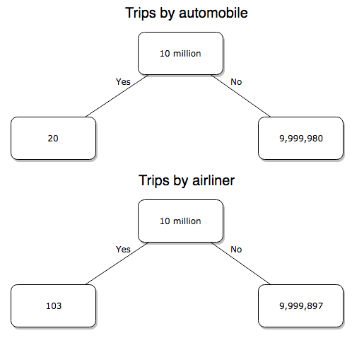
Figure 2. A probability tree to help visualize comparison of deaths (“yes”) by car travel and by airline travel in the United States for the year 2000.
Comparing rates and proportions
Without going into the details, we will do so in Chapter 9 Inferences on Categorical Data, comparing two rates is a chi-square, χ2, contingency table type of problem. More specifically, however, it is a binomial problem (Chapter 3.1, Chapter 6.5); there are two outcomes, death or no death, and we can describe how likely the event is to occur as a proportion. Because the numbers are large, we can use rely on the normal distribution for comparing the two proportions. We’ll explain this more in the next chapters, but for now it may be enough to present the equation for the comparison of two proportions under the assumption of normality, proportion z test.
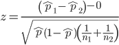
and the null hypothesis (see Chapter 8) tested as that the two proportions are equal. This may be written as
H0 : p1-p2=0
We can assign statistical significance to the differences in events for the two modes of travel under this set of assumptions. Rcmdr has a nice menu-driven system for comparing proportions, but for now I will simply list the R commands.
At the R prompt type each line then submit the command.
total = 100000000
prop.test(c(19700,14),c(total,total)))
And the R output
prop.test(c(19700,14),c(total,total))

    2-sample test for equality of proportions with continuity
    correction

data:  c(19700, 14) out of c(total, total)
X-squared = 19658, df = 1, p-value < 2.2e-16
alternative hypothesis: two.sided
95 percent confidence interval:
 0.0001940984 0.0001996216
sample estimates:
  prop 1   prop 2
1.97e-04 1.40e-07
There’s a bit to unpack here. R is consistent; when it reports results of a statistical test, it typically returns the value of the test statistic (χ2 = 19658), the degrees of freedom for the test (df = 1), and the p-value (< 2.2e-16).
prop.test() were calculated by the Wilson Score method not the Wald method. While both are parametric tests and therefore sensitive to departures from normality (see Chapter 13.3), formulation of Wilson score method makes fewer assumptions (involving approximations of the population proportions) and therefore is considered more accurate.By convention in statistics, if a p-value, where “p” stands for probability, is less than 5%, we would say that our results are statistically significant from the null hypothesis. Looks pretty convincing to me, the difference of 19,700 deaths compared to 14 deaths is clearly different by any criterion and by the results of the statistical test, the p-value is several orders of magnitude smaller than 5%.
Safer to fly. By far, not even close. And similar conclusions would be reached if we compare different years, or averages over many years, or if we used a different way to express the amount of travel (eg, miles/year) by these modes of transportation.
Are you convinced, really? Is it safer to fly?
Let’s try a little statistical reasoning — what assumptions did I make to do these calculations? We recognize immediately that many more people travel by car: that there are way more cars being driven then there are airline planes being flown. The question then is, have we properly adjusted for this difference? Here are a few considerations. My source for the numbers is the NTS 2001 book published by the U.S. Department of Transportation (U.S. Department of Transportation). We are conducting a risk analysis, and the first step is to make sure that we are comparing “apples with apples.” Here are two alternative solutions that at least compare, “Red Delicious” apples with “Macintosh” apples.
Option 1. There are many, many more licensed drivers than there are licensed commercial airline pilots. The standard comparison offered in the background above compared deaths per licensed car driver, but a different metric for air travel, the rate per passenger. This isn’t as bad of a comparison as it may seem — after all, the majority of deaths in car accidents are of the driver themselves. But it isn’t that hard to make the direct comparison — just find out how many commercial pilots there are — a direct comparison with licensed car drivers (stated above as 190,625,023). From the FAA we see that in 2009 there were 125,738 persons with commercial certificates. Since there are only 20 major airline carriers in the United States now (a few more were active in 2000, but we’ll put this aside), the number of licenses is an over estimate of the actual number we want — how many pilots of commercial airlines — but lets use this number for starters — after all, just because a person has a drivers license doesn’t mean they drive or ride in a car.
Number of deaths/yr: Let’s use 2000 data, a typical year prior to 9/11 (and excluding the Covid-19 pandemic). Airlines: 92 deaths; motor vehicles (includes passenger cars, trucks, etc, but not motorcycles): 37,526 deaths (drivers = 25,567; passengers = 10,695; 86 others).
Which mode of travel is riskier? I get a rate a rate of 7.3 X 10⁻⁴ deaths per commercial pilot, or
92125738
compared to a rate for car drivers of 1.97 X 10⁻⁴ deaths.
To summarize what we have so far, I get a result that suggests car travel is almost four times safer
7.3 x 10-41.97 x 10-4→7.31.97 = 3.7
then traveling by commercial airliner. In whole numbers, these results translate to seven deaths for every 10,000 commercial pilots compared to two deaths for every 10,000 licensed car drivers (Fig 3).
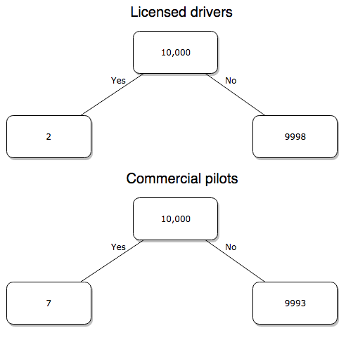
Figure 3. Comparing totals of deaths adjusted by numbers of licensed drivers and by licensed commercial airline pilots in the United States.
R work follows. Enter and submit each command on a separate line in the script window
total = 10000
prop.test(c(2,7),c(total,total))
And the R output
prop.test(c(2,7),c(total,total))

    2-sample test for equality of proportions with continuity
    correction

data:  c(2, 7) out of c(total, total)
X-squared = 1.7786, df = 1, p-value = 0.1823
alternative hypothesis: two.sided
95 percent confidence interval:
 -0.001187816  0.000187816
sample estimates:
prop 1 prop 2
 2e-04  7e-04
What’s happened? The p-value (0.1823) is not less than 5% and so we would conclude under this scenario that there is no difference between the proportions of deaths between the two modes of travel. Let’s keep going.
Option 2. There are many, many more cars on the road then there are airplanes flying commercial passengers. The standard comparison offered in the background information above identified death rates per individual driver, but used a different metric for airline travelers (number of deaths per passenger), which confuses individuals with travelers: what we need is the number of individuals that traveled by airliner, not the total number of passengers (which is many times higher, because of repeat flyers). How can we make a fair comparison for the two modes of travel? Most people never fly whereas most people drive (or ride in a car) frequently in the United States. To me, risk of travel might be better expressed in terms of a per trip rate. I want to know, what are my chances of dying each time I get into my car versus each time I fly on a commercial jet in the United States?
Number of trips/yr. For airlines, I use the number of departures (2000 = 8,951,773). But for cars, we need to decide how to get a similar number. It’s not available directly from the DOT (and would be difficult to get — studies with randomly selected drivers can yield as many as 5 trips per day for licensed drivers). I took the number of licensed drivers and bound the problem — at the low end, let’s say that only 2 trips per week (eg, 50 weeks) are taken by licensed drivers (100 trips); at the upper end, let’s take 2 trips per day per week, or 500 trips/year. Thus, at the low end, we have 1.91 X10¹⁰ trips per year; at the upper end, 9.53 X 10¹⁰ trips per year.
Which mode of travel is riskier? Using the number of deaths/yr listed above in Option 1, I get a rate of 1.03 X 10⁻⁵ deaths/trip for air carriers
928.95 x 10⁶
compared to a rate of 1.97 X 10⁻⁶ deaths/trip for cars (lower bound) or 3.9 X 10⁻⁷ deaths/trip for cars (upper bound). Here’s what the numbers look for in a tree (taking the lower number of trips per year for cars, Fig 4).
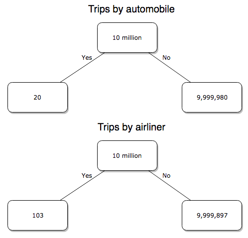
Figure 4. Comparing totals of deaths adjusted by numbers of car trips and by numbers of airline trips in the United States.
R work follow
total = 10000000
prop.test(c(20,103),c(total,total))
And the R output
prop.test(c(20,103),c(total,total))

    2-sample test for equality of proportions with continuity
    correction

data:  c(20, 103) out of c(total, total)
X-squared = 54.667, df = 1, p-value = 1.428e-13
alternative hypothesis: two.sided
95 percent confidence interval:
 -1.057370e-05 -6.026305e-06
sample estimates:
  prop 1   prop 2
2.00e-06 1.03e-05
Now we have another really small p-value (1.428e-13), which suggests a statistically significant difference between the modes of air travel, but the difference in deaths is switched. I now have a result that suggests car travel is much safer than traveling with a commercial airliner! These calculations suggest that you are as much as 26 (upper bounds, five times for lower bounds) times more likely to die from a plane crash then you are behind the wheel. In whole numbers, these results indicate one death for every 100,000 airline flights compared to 1 death for every 500,000 (lower estimate) or 2,500,000 car trips!
Do I have it right and the standard answer is wrong? As Lee Corso used to say on ESPN’s College GameDay program, “Not so fast, my friend!” (Wikipedia). Mark Twain was right to hold the skeptic’s view. Begin by listing the assumptions and by checking the logic of the comparisons (there are still holes in my logic!!). For one, if I am considering my risk of dying by mode of travel, it is far more likely that I will be in a car accident than I will an airline accident, simply because I don’t travel by airline that much. When we consider lifetime risk, we can see why the assertion that it is “safer to fly than drive” is true — we’re far more likely to belong to one of the reference populations involving automobiles (eg, those who drive frequently, for many years) than we are to be among the frequent flyers reference populations.
Questions
1. Review and provide your own examples for
- index
- rate
- ratio
- proportion
3. Like travel safety, we are often confronted by risk comparisons like the following: Which animal is more deadly to humans, dogs or sharks? Between the two, which lead to more hospitalizations in the United States? Work through your assumptions and use results from the International Shark Attack file.
- If a person lives in Nebraska, and never visits the ocean, how does a “shark attack” risk analysis apply? Is it a fair comparison to make between dog attacks and shark attacks? Why or why not.
4. Go to cappex.com/colleges and update institutional (gift) aid offered by Chaminade and HPU. Compare to University of Hawaii-Manoa.
5. Calculate percent increase for
- Annual atmospheric CO2 1980 and 2024.
Quiz Chapter 6.2
Ratios and probabilities
Chapter 6 content
- Introduction
- Some preliminaries
- Ratios and probabilities
- Combinations and permutations
- Types of probability
- Discrete probability distributions
- Continuous distributions
- Normal distribution and the normal deviate (Z)
- Moments
- Chi-square distribution
- t distribution
- F distribution
- References and suggested readings
11.4 – Two sample effect size
Introduction
An effect size is a measure of the strength of the difference between two samples. Effect size tells us the practical importance of a result, say, the difference in outcome between a control group and the treatment group. A combined effect size is a common goal of any meta-analysis (Chapter 20.15).
Note 1: To calculate a combined effect size in meta-analysis, pool individual study effect sizes into a single summary effect. If sample size differs widely across the studies, use a weighted average. Thus, studies with more precision get more weight.
By including effect sizes, this complement inferential statistics such as p-values. Importantly, effect size moves us beyond “significant” or “not significant.” Significance tells us a difference is likely between the groups, but offers no information about the practicality of the observed difference. After all, large studies inherently have more statistical power, which, by definition implicates even small differences can be statistically significant.
In statistics there are many estimates of effect size: for categorical data, odds ratio and relative risk between exposed and unexposed groups; for quantitative data, correlation, regression slope are effect size measures, in addition to the difference between group means. For differences in means between groups, Cohen’s d (and Hedge’s g) are common statistics. In ANOVA, eta-squared ( ) and omega-squared (
 ), summarizes the proportion of total variance in the dependent variable explained by the independent variables while
 the coefficient of determination, represents the proportion of variance in the outcome explained by the predictors. Advice and help for understanding “effect size” is an enormously popular topic — nearly 3 million hits in Google Scholar and about forty-five thousand papers in Pubmed. Two highly cited papers are those by Durlak (2009) and Ferguson (2009).
The effect size statistic, Cohen’s d, is calculated by subtracting one sample mean from the other and dividing by the pooled standard deviation.
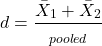
where spooled is the pooled standard deviation for the two sample means.
Hedge’s d, which uses the spooled is the pooled standard deviation for the two sample means instead of the pooled population standard deviation, is written as
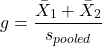
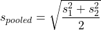
The  used in d is from an equation for pooled standard deviation was provided in Chapter 3.3, but we’ll give it again here.
An alternative version of Cohen’s d is available for the t-test test statistic value

A d of one (1) indicates the effect size is equal to one standard deviation; a d of two (2) indicates the effect size between two sample means is equal to two standard deviations, and so on.
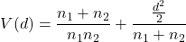
The variance of Cohen’s d,  , can be estimated as
Hedges’ g (Hedges 1981), which includes a Bessel’s correction for bias in small samples, includes “ in the denominator of the pooled standard deviation calculation.
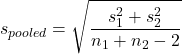
The “-2” forces the pooled variance to be larger — that makes g more conservative than d, which is of use for small sample studies.
A simple modification converts d to g. Multiple d by a small-sample size correction factor J (Durlak 2009):
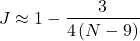
Note 2: Fall 2025 update: this section is actively being modified to better reflect what Cohen, Hedges, and others actually meant. In particular, formulas presented here should be considered as provisional awaiting confirmation and improvements to better reflect historical definitions and modern implementations.
What makes a large effect size?
Cohen cautiously suggested that values of d can be interpreted as
0.2 – small effect size
0.5 – medium effect size
0.8 – large effect size
That is, if the two group means don’t differ by much more than 0.2 standard deviations, than the magnitude of the treatment effect is small and unlikely to be biologically important, whereas a d = 0.8 or more would indicate a difference of 0.8 standard deviations between the sample means and, thus, likely to be an important treatment effect. Cohen (1992) provided these guidelines based on the following argument. The small effect 0.2 comes from the idea that it is much worse to conclude there is an effect when in fact there is no effect of the treatment rather than the converse (conclude no effect when there is an effect). The ratio of the Type II error (0.2) divided by the Type I error (0.05) gives us the penalty of 4. Similarly, for a moderate effect,  equals 10. Clearly, these are only guidelines (see Lakens 2013).
Examples
The difference in average body size between six week old females of two strains of lab mice is 0.4 g (Table 1), and increases to 1.38 g by 16 weeks (Table 2).
Table 1. Average body weights of 6 week old female mice of two different inbred strains.†
| Strain |  |
s |
| C57BL/6J | 18.5 | 0.9 |
| CBA/J | 18.1 | 1.27 |
†Source: Jackson Laboratories: C57BL/6J; CBA/J
Table 2. Average body weights of 16 week old female mice of two different inbred strains.†
| Strain | |
s |
| C57BL/6J | 23.9 | 2.3 |
| CBA/J | 25.38 | 3.76 |
†Source: Jackson Laboratories: C57BL/6J; CBA/J
The descriptive statistics are based on weights of 360 individuals in each strain (Jackson Labs).
The differences are both statistically significant from a independent t-test, i.e., p-value less than 0.05. I’ll show you how to calculate independent t-test given summary statistics (means, standard deviations), for Table 1 data, then will ask you to do this on your own in Questions.
Write an R script, example data from Table 1
sdd1 = 0.9
var1 = sdd1^2
sdd2 = 1.27
var2 = sdd2^2
mean1 = 18.5
mean2 = 18.1
n1 = 360
n2 = 360
dff = n1+n2-2
pooledSD <-sqrt((var1+var2)/2)
pooledSEM <-sqrt(var1/n1 + var2/n2); pooledSEM
tdiff<-(mean1-mean2)/pooledSEM; tdiff
pt(tdiff, df=dff, lower.tail=FALSE)
#get two-tailed p-value
2*0.0000006675956
#get cohen's d
2*tdiff/sqrt(dff)
Results from the calculations we report (value of the test statistic, degrees of freedom, p-value), and the effect size, then are
t = 4.875773, df = 718, p-value = 0.0000006675956
cohen's d = 0.364
Now, I’m from the school of “don’t reinvent the wheel” or “someone has already solved your problems” (Freeman et al 2008), when it comes to coding problems. And, as you would expect, of course someone has written a function to calculate the t-test given summary statistics. In addition to base R and the pwr package (see Chapter 11.5), the package BSDA contains several nice functions for power calculations.
To follow this example, install BSDA, then run the following code
require(BSDA)
tsum.test(mean1, sdd1, n1, mean2, sdd2, n2, alternative = "two.sided", mu = 0, var.equal = TRUE, conf.level = 0.95)
R output
Standard Two-Sample t-Test

data: Summarized x and y
t = 4.8758, df = 718, p-value = 0.000001335
alternative hypothesis: true difference in means is not equal to 0
95 percent confidence interval:
0.2389364 0.5610636
sample estimates:
mean of x mean of y
18.5 18.1
Similarly, Cohen’s d is available from a package called effsize.
Note 3: One reason to “re-invent the wheel,” I only needed the one function; the BSDA package contains more 330 different objects/functions. A simple way to check how many objects in a package, eg, BSDA, run
ls("package:BSDA")
BSDA stands for “Basic Statistics and Data Analysis,” and was intended to accompany the 2002 book of the same title by Larry Kitchens.
And of course, if using some else’s code, give proper citation!
Questions
- We needed an equation to calculate pooled standard error of the mean (
pooledSEMin the R code). Read the code and write the equation used to calculate the pooled SEM. - Calculate the t-test and the effect size for the Table 1 data, but at three smaller sample sizes. Change from 360 for n1 = n2 = 20, repeat for n1 = n2 = 50, and finally, repeat for n1 = n2 = 100. Use your own code, or use the
tsum.testfunction from theBSDApackage. - Calculate Cohen’s effect size d for each new calculation based on different sample size.
- Create a table to report the p-values from the t-tests, the effect size, for each of the four n1 = n2 = (20, 50, 100, 360).
- True or false. The mean difference between sample means remains unaffected by sample size.
- True or false. The effect size between sample means remains unaffected by sample size.
- Based on comparisons in your table, what can you conclude about p-value and “statistical significance?” About effect size?
- Repeat questions 2 – 7 for Table 2.
Quiz Chapter 11.4
Two sample effect size
Chapter 11 contents
11.2 – Prospective and retrospective power
Introduction
Statistical power is defined as p = 1 – β. The power of a test is the probability of rejecting a Null Hypothesis when it is false. There is a relationship between Type I error and Type II error. We want β to be Large BUT β is generally not known when we are performing the statistical test. We do know that α is inversely related to β. The smaller the α value we use to Reject the Null Hypothesis the MORE likely we will accept a FALSE Null Hypothesis. If we make α very small (one in a billion) then there would be a very HIGH chance of accepting α Null Hypothesis when it is false (β is high). Note that this is the same discussion that we had about sensitivity of an assay test and the specificity of that assay. If we increase sensitivity of the assay such that we approach 100% detection of the true positives will be detected, we necessarily will increase the number of false positives. The BEST way to reduce both Type I and Type II statistical errors is to INCREASE the sample size!
Power of any statistical test (Z test, T-test, one-way ANOVA…) can be determined BEFORE the experiment is done and data are gathered or AFTER an experiment is completed (Cohen 1992). For now, here’s our first real taste of experimental design — we can evaluate how we can make an experiment to test a particular hypothesis.
Prospective power analysis
Good experimental design should include considerations of power. The design will determine the size of the effect your experiment will be able to detect and the probability of correctly rejecting the null hypothesis. In large part, this will involve decisions of sample size and ways to reduce error variance. Moreover, one needs to decide ahead of time, just how large of an effect does the experiment need to detect??? A one-gram change in body mass before and after a diet treatment is of no concern whatsoever if your study subjects are African elephants, but may be a very large effect for a study of shrews!
Retrospective power analysis
Power analysis can also be done after a test has been conducted and the null hypothesis failed to be rejected. One interpretation that might follow from a retrospective power analysis is that, if the study had low power, the lack of statistical significance could be viewed merely the result of low sample size. However, as forcefully argued Hoenig and Heisey (2001) (see also Colegrave and Ruxton 2003), retrospective or posthoc power tests provide no more information than does the p-value and therefore are redundant. At worse, retrospective power analysis can be misleading as to how well it predicts true power, ie, biologically meaningful differences between different treatment groups (Zhang et al., 2019).
Prospective power is more than effect size between groups
Large effect size, ie, large differences between groups, is not necessarily evidence of important biological differences. The concept of power has limits (Hoenig and Heisey 2001 Yuan and Maxwell 2005). On the other hand, small effect sizes can be important differences, especially if the treatment is difficult or expensive. We work through this conclusion with an example, but emphasize here that providing confidence intervals for the effect size (Colegrave and Ruxton 2003). Suppose the null hypothesis was not rejected from a two sample independent t-test conducted on the test of differences in plant height between two samples of `ohi’a found at different elevations. Was there really no difference or was the sample size in the study simply too small to detect the real and important difference between the samples? By conducting a power analysis, one can determine if a slight increase in sample size would have yielded a statistically significant difference, or it may suggest that the effect size is small enough not to warrant further attention.
R code
Three options for conducting power analysis in R are provided in section 11.5
Questions
- Assuming that a study was done by randomly sampling from a population, and the the primary outcome is found not statistically different with p-value 0.13 between placebo and treatment groups, what can be gained made from a retrospective power analysis?
Quiz Chapter 11.2
Prospective and retrospective power
Chapter 11 contents
- Introduction
- What is Statistical Power?
- Prospective and retrospective power
- Factors influencing statistical power
- Two sample effect size
- Power analysis in R
- References and suggested readings
10.1 – Compare two independent sample means
Introduction
We introduced the concept of comparing a sample statistic (mean) against a population parameter (Chapter 6.7, Normal deviate) or one-sample t-test against a specified mean (eg, from published data or from theory, Chapter 8.5).
Consider now a basic experimental design, the randomized control trial, or RCT (Fig 1), introduced in Chapter 2.4.
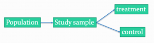
Figure 1. A two group Randomized Control Trial.
Subjects randomly selected from population of interest, then again — random assignment — once recruited into one of two treatment groups. Importantly, subjects belong to one treatment arm only: no subject simultaneously receives the treatment and the control. This is in contrast to the paired design, in which subjects receive both treatments (see Chapter 10.3).
In inferential statistics about an experiment, we are more likely trying to test if sample means are different. For example
- two species grown in common garden, do they differ in growth rate?
- human subjects given a new treatment have better outcomes compare to those receiving a control treatment (eg, placebo).
The equivalent null hypothesis is that two samples are pulled from the same population. We write the null hypothesis as

and the corresponding alternative hypothesis, HA, then must be

Question: Is this a one tailed or two-tailed hypothesis?
Answer: Two-tailed (review Chapter 8.4)
Note 1: In this day and age, there’s really no compelling reason to learn the t-test. First, it is just a special case of the one-way ANOVA, therefore, it’s a special case of the general linear model. Struggling to learn R commands? Well, one solution would be just to learn the general linear model approach — the R function lm() (OK — don’t get too excited — lm() has many options and details). Second, few experiments or observational studies are likely to have only two groups; thus, the temptation to carry out a series of t-tests, taking all groups two at a time, or “pairwise,” while tempting, actually violates a whole bunch of basic statistical rules (discussed in Chapter 12.1). It will also make statisticians go crazy when they see it. That said, if your experiment has but two groups, then by all means, the t-test is a choice. The t-test is also a statistical test that you have likely already used before so we present the discussion here to build on what you may already have learned. We also present the independent t-test as a vehicle.
Worked example
We introduce the two-sample t-test, or better, the independent sample t-test.

where the numerator is the difference between the two sample means and the denominator is the standard error of the differences between the two groups standard errors. The formula for
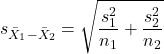
The choice of independent sample over two-sample is best because it emphasizes that the two groups (the two samples), must be comprise of independent sampling units. This is a pretty straight-forward requirement; you have randomly assigned twenty individuals to two groups, a control group (n = 10) and a treatment group (n = 10). Individuals are either in the control group or they are in the treatment group — they cannot simultaneously appear in both groups.
We will work our way through this test by example. For starters, let’s use the same lizard dataset (see Example data set, below), four body mass recordings (grams) each for house geckos (Hemidactylus frenatus, Fig 2) and the Carolina anole (Anolis carolensis, Fig 3), two of many lizard species introduced to Hawaiʻi.

Figure 2. Male Hemidactylus frenatus, central Oahu, M. Dohm.

Figure 3. Male Anolis carolinensis, ʻAkaka Falls, Big Island of Hawaiʻi, M. Dohm.
Example data set
Geckos: 3.186, 2.427, 4.031, 1.995

Anoles: 5.515, 5.659, 6.739, 3.184
Question: How would you go about creating a data frame with the values in long form (stacked worksheet), including a label variable and the body mass?
Note 2: The independent sample t-test in Rcmdr requires a stacked worksheet and not in unstacked worksheet two columns implied by the above pseudo-code. If you need help with worksheet format, then see Part07 in Mike’s Workbook for Biostatistics.
Answer: At the R prompt, type
Geckos <- c(3.186, 2.427, 4.031, 1.995); Anoles = c(5.515, 5.659, 6.739, 3.184) #create two vectors
bmass <- c(Geckos, Anoles)    #combine the two vectors into a single vector holding all of the body mass records
species <- c("gecko", "gecko", "gecko", "gecko", "anole", "anole", "anole", "anole")   #create your label variable
lizards <- data.frame(species, bmass)  #create your data frame
lizards   #print your data frame  species bmass
1   gecko 3.186
2   gecko 2.427
3   gecko 4.031
4   gecko 1.995
5   anole 5.515
6   anole 5.659
7   anole 6.739
8   anole 3.184
Note also that you can enter data into the Data editor by creating the data frame first then adding values. To edit the data frame “lizards” type fix(lizards) at the R prompt, then close the data frame when you have added or changed values as needed.
As always, begin with an exploration of the data, including a graph (Fig 4).
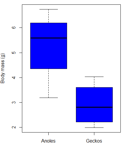
Figure 4. Box plot of lizard body mass.
We can see already that there’s greater spread of data for the Anoles compared to the Geckos, but the median values differ. Small sample sizes can be a problem for analyses as we can only have reduced confidence in our conclusions. However, we press on for the sake of demonstration.
Let’s test the null hypothesis, H0, ie, the two species of lizards have the same mean body mass.
Rcmdr: Statistics → Means → Independent-samples t-test…
In this next image I posted the Rcmdr menu popup for the Independent Samples t-test (Fig 5). Later versions of Rcmdr split the settings for this command into two tabs; the first tab allows for the selection of the variables and setting the hypotheses whereas the second tab, labeled Options, permits additional choices. The default selections need your attention: to actually conduct the t-test you need to answer “No” to the question, “Assume equal variance?” (Fig 6).
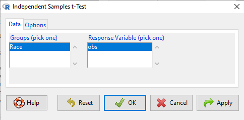
Figure 5. Rcmdr menu for Independent sample t-test.
Select the Options tab (Fig 6) to select null hypothesis and to select the t-test and not the Welch-test (which is the default, ie, No to the prompt “Assume equal variances?”).
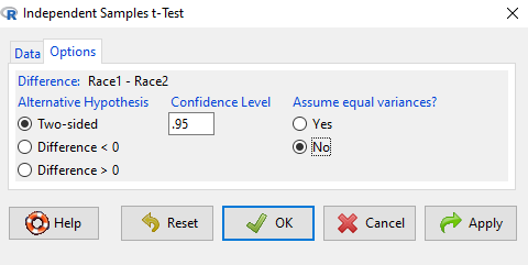
Figure 6. Rcmdr Options menu for Independent sample t-test.
Let’s look at the results and break down the parts of the test.
t.test(Body.mass~Lizard, alternative='two.sided', conf.level=.95,
+ var.equal=TRUE, data=lizards)

Two Sample t-test

data: Body.mass by Lizard
t = 2.7117, df = 6, p-value = 0.03503
alternative hypothesis: true difference in means is not equal to 0
95 percent confidence interval:
0.2308685 4.4981315
sample estimates:
mean in group Anolis mean in group Gecko
5.27425 2.90975
Consider the R session output above and answer the following questions.
Questions for the worked example
- Which lizard group had the greater mean value, Anolis or Gecko?
- What are the assumptions necessary for you to use the independent sample t-test?
- What does “two-sided” mean?
- What was the null hypothesis?
- Was this a one-tailed or two-tailed test of the null hypothesis?
- What is the value of the test statistic?
- How many degrees of freedom?
- What is the critical value for this test?
- What is the value of the lower limit of the 95% confidence interval?
- What is the value of the lower limit of the 99% confidence interval?
- True or False. If the null hypothesis is accepted, then zero is a value included in the 95% confidence interval.
- Do you accept the null hypothesis? Explain your selection.
Try another example
DNA damage, changes in the chemical structure of nucleotide bases or breakage of the DNA chains, occurs in cells under many circumstances. The comet assay, or single-cell gel electrophoresis, is one method for visualizing and measuring DNA strand breaks in cells. Exposed cells are mixed with a low-melting temperature agarose and placed onto a microscope slide. The cells are then lysed with an alkaline detergent and high salts. When current is applied across the slide, undamaged DNA remains in the nucleus, whereas damaged DNA extends towards the anode to form a comet-like tail, with imaging assisted by including a fluorescent dye like Sybr-Green. Examples of comets are shown below (Fig 7).
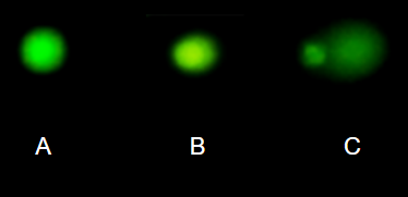
Figure 7. Comet examples. A Intact cell, no DNA damage, B Cell with some DNA damage, a slight tail to the right is evident, C Cell with significant DNA damage, a large tail is evident. M. Dohm.
In an experiment, immortalized lung epithelial cells were exposed to dilute copper solutions for 30 minutes then washed with PBS. The comet assay was applied to these cells and for comparison, to cells without copper exposure but otherwise treated the same way (controls). The data are available at the bottom of this page (scroll down or click here).
Again, you should begin all analyses with an exploration of the data, including a graph (Fig 8).
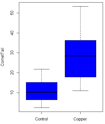
Figure 8. Boxplot of comet tail lengths for cells with and without (control) exposure to copper in the cell medium for 30 minutes.
Let’s look at the R output for the t-test analysis.
    Two Sample t-test

data:  CometTail by Treatment
t = -5.8502, df = 38, p-value = 9.139e-07
alternative hypothesis: true difference in means is not equal to 0
95 percent confidence interval:
 -22.39865 -10.88213
sample estimates:
mean in group Control  mean in group Copper
             11.14533              27.78571
Consider the R session output above and answer the following questions.
Questions for Comet assay data set
- Which cell group had the greater mean value, Copper-exposed or Control-exposed cells?
- What are the assumptions necessary for you to use the independent sample t-test?
- What does “two-sided” mean?
- What was the null hypothesis?
- Was this a one-tailed or two-tailed test of the null hypothesis?
- What is the value of the test statistic?
- How many degrees of freedom?
- What is the critical value for this test?
- What is the value of the lower limit of the 95% confidence interval?
- What is the value of the lower limit of the 99% confidence interval?
- True or False. If the null hypothesis is accepted, then zero is a value included in the 95% confidence interval.
- Do you accept the null hypothesis? Explain your selection.
T test from summary statistics
In some cases you may only have to summary statistics for data, eg, the means and the standard deviations. We can use the equations of the t test to write a simple formula, where the user provides the known means, standard deviations, and sample size. For example, create a simple function with readline for user input.
myTtest <- function() {
   mnx <- as.numeric(readline(prompt="Enter mean of x: "))
   stdevx <- as.numeric(readline(prompt="Enter sd of x: "))
   nx <- as.numeric(readline(prompt="Enter n of x: "))
   mny <- as.numeric(readline(prompt="Enter mean of y: "))
   stdevy <- as.numeric(readline("Enter sd of y: "))
   ny <- as.numeric(readline(prompt="Enter n of y: "))
   myTvalue <- abs(((mnx-mny)-0)/sqrt(((stdevx^2)/nx)+(stdevy^2)/ny))
   myDF <- as.integer(nx+ny-2)
   myPvalue <- pt(myTvalue,myDF,lower.tail=FALSE)*2
   myResults <- c(myTvalue, myDF, myPvalue)
   report <- c("T-test: ", "df: ", "two-tailed p-value: ")
   cat(sprintf("%s %3.3f, ", report, myResults))
}
then run the function by typing myTest() at the R prompt and entering the means, standard deviations, and sample size when prompted.
myTtest()
Enter mean of x: 2.91
Enter sd of x: .895
Enter n of x: 4
Enter mean of y: 5.27
Enter sd of y: 1.497
Enter n of y: 4
T-test: 2.706, df: 6.000, two-tailed p-value: 0.035
P-values from confidence intervals
While we expect certain reporting criteria for published, it is not uncommon that one or more elements are missing. For example, while means plus or minus standard deviations for two groups may be reported, the confidence interval of the difference may not be reported, or, an inexact p-value is reported like “< 0.05,” but we “need” an exact p-value for our meta-analysis. A little math, and these missing statistics can be calculated.
We can use the lizard study as an example; while all of the expected elements were reported, including the p-value (0.03503), let’s say the p value was reported as “statistically significant at p < 0.05.”
We need
lower and upper confidence intervals: 0.2309 and 4.498, respectively.
critical value from t distribution, df = 6 (2 tailed, therefore 0.05/2). A little R code we have:

the standard error, which can be calculated as 
and then the p-value, 
which is pretty close to the result from R (p = 0.03503). The difference is likely due to the small sample size.
Questions
- Don’t forget to work through the Questions for the Comet tail data set (scroll up or click here).
- Microsoft Excel, LibreOffice Calc, and Google sheets spreadsheet software all include t-test functions and return the p-value. Consider two variables big (100, 110, 120, 100, 110, 210, 200) and small (0,1,1,2,0,1,0). (Note — these two groups are obviously very different, calculating a t-test on their difference is silly, just for this question.) If formatting is set to the default two decimal places for Number cell category, the p-value will return as “0.00.” How should you report the p-value in this case?
Quiz Chapter 10.1
Compare two independent sample means
Comet assay data set
| Treatment | CometTail |
| Control | 17.856139 |
| Control | 16.52125 |
| Control | 14.925449 |
| Control | 14.029174 |
| Control | 13.332945 |
| Control | 8.811185 |
| Control | 14.701654 |
| Control | 9.261025 |
| Control | 21.779311 |
| Control | 6.180284 |
| Control | 9.201752 |
| Control | 5.54472 |
| Control | 6.717885 |
| Control | 2.625092 |
| Control | 7.191583 |
| Control | 5.392866 |
| Control | 11.284813 |
| Control | 15.441254 |
| Control | 17.857176 |
| Control | 4.250956 |
| Copper | 53.214287 |
| Copper | 38.92857 |
| Copper | 18.928572 |
| Copper | 30 |
| Copper | 28.928572 |
| Copper | 15.357142 |
| Copper | 17.857143 |
| Copper | 17.5 |
| Copper | 21.071428 |
| Copper | 29.285715 |
| Copper | 28.214285 |
| Copper | 16.785715 |
| Copper | 21.071428 |
| Copper | 37.5 |
| Copper | 38.214287 |
| Copper | 17.857143 |
| Copper | 29.642857 |
| Copper | 11.071428 |
| Copper | 35 |
| Copper | 49.285713 |
Chapter 10 contents
- Introduction
- Compare two independent sample means
- Digging deeper into t-test Plus the Welch test
- Paired t-test
- References and suggested reading
9.4 – Heterogeneity chi-square tests
Planned comparisons and meta-analysis.
After finding evidence to reject the statistical null hypothesis, it may be appropriate to proceed to test a number of data sets against the same theoretical distribution. Provided these are planned comparisons, part of the experiment and not an exercise in data dredging (Norman 2014), you may proceed to test a series of nested models where groups are combined to make new groups for comparison. This approach is analogous to the post-hoc tests one may conduct after a statistically significant ANOVA (see Chapter 12.4) or when identifying a best-fit regression model (see Chapter 18.4).
Combining groups to make new comparisons — this scenario is consistent with a meta-analysis. A type of systematic review (Greenhalgh 1997, Akobeng 2005), meta-analysis is a statistical method that combines the results from multiple independent studies on the same topic to provide a more precise and robust overall conclusion. By combining studies, the goal is to calculate a pooled estimate as a measure of overall effectiveness of the treatment. Meta-analysis can increase the overall sample size, which improves the study’s ability to detect an effect if one exists. So, how to combine results from different studies ostensibly addressing the same hypothesis? Inevitably, some subjectivity will come into decisions about including or excluding studies — the goal is to identify quality studies, which may have conflicting conclusions and test whether a single conclusion of effectiveness is warranted based on a summary of evidence.
Here we introduce the Cochran’s Q test (Cochran 1954, Hoaglin 2016), aka a special case of the more general heterogeneity chi-square test. The null hypothesis is no significant difference in the proportion of “successes” across all groups being compared — any observed differences between the groups are just due to chance. The test statistic, Q, has a chi-square distribution with  degrees of freedom. A large Q value and small p-value suggest significant heterogeneity of results among the studies.
Note 1. As a reminder, “success” as an outcome category in epidemiology studies can represent any result depending on the study’s objective: survival, recovery, symptom improvement, or prevention of infection. The alternative outcome is generally referred to as “failure” (eg, death, non-recovery, no improvement, infection).
Heterogeneity tests ask whether results from combined studies are consistent; other tests exist, and are detailed in our special chapter on conducting meta-analysis. For example, I2 or I-squared test provides a measure of how much variation in the combined studies is due to true differences rather than by chance. In short, the I2 test quantifies how much — the percentage — the different studies agree, while the chi-square test returns a p-value that can be used to interpret whether that heterogeneity is statistically significant. We outline the basics of meta-analysis in Chapter 20.15. Other tests include DerSimonian-Laird test and Mandel-Paule test — these use the Q statistic and its distribution to estimate the between-study variance and provide better estimators with small sample size. Between-study variance is used to determine if a fixed-effect or a random-effects model (Chapter 12.3 and Chapter 14.3), is appropriate for the analysis. A random-effects model is used when significant heterogeneity is present (Higgins et al 2009).
Example.
Imagine a scenario where a population geneticist has collected allele (gene) frequency and genotype frequency data on single nucleotide polymorphisms (SNP) for the BRCA1 locus for three USA groups, African Americans, Asian Americans, and European Americans. Data of this kind can be obtained from the SNP database at NCBI (data retrieved 14 & 15 July 2014), and I collated several SNP involving a Cytosine base for Thymine base change (Table 1). The BRCA1 locus is on chromosome 17 and some of the hundreds of mutations found for this gene are associated with high risk of breast and or ovarian cancer (Couch and Weber 1996, Tram et al 2013).
Table 1. SNP of BRCA1 locus
| SNP | Population | n | C/C | C/T | T/T | C | T |
| rs1060915 | African American | 46 | 0.043 | 0.174 | 0,783 | 0.130 | 0.870 |
| Asian American | 48 | 0.083 | 0.625 | 0.375 | 0.396 | 0.604 | |
| European American | 48 | 0.167 | 0.458 | 0.375 | 0.396 | 0.604 | |
| rs3737559 | African American | 40 | 0.043 | 0.174 | 0.783 | 0.130 | 0.870 |
| Asian American | 48 | 0.083 | 0.625 | 0.292 | 0.396 | 0.604 | |
| European American | 48 | 0.167 | 0.458 | 0.375 | 0.396 | 0.604 | |
| rs799917 | African American | 124 | 0.048 | 0.258 | 0.694 | 0.177 | 0.823 |
| Asian American | 90 | 0.467 | 0.444 | 0.089 | 0.689 | 0.311 | |
| European American | 118 | 0.407 | 0.458 | 0.136 | 0.636 | 0.364 |
We may wish to test the combined data set to see if the large data set differs from Hardy Weinberg expectations before proceeding with a series of sample populations. By combining the data sets, we will be able to test whether one genotype is different from exception.
The goal then is to pool the data so that you have a more powerful test of the null hypothesis (remember our general discussion of statistical power and how increasing sample size increases your chances of correctly rejecting the null hypothesis).
For example, in our test of Hardy-Weinberg expectations (Example C), we calculated a  test of 7.8955. This test has k – 1 = 3 – 1 = 2 degrees of freedom. At alpha 5%, the critical value was 5.991 We clearly would reject the null hypothesis. But do we reject because of a difference in the aa, ab, or bb genotypes? Simply combine categories. Let’s test the homozygotes (aa and bb) versus the heterozygotes (ab).
Table 2. Worksheet
|
Categories
|
|||
| aa + bb | ab | n | |
|
Observed
|
66 | 34 | 100 |
|
Expected
|
52 | 48 | 100 |
 |
 |
||
With one degree of freedom, we clearly reject the null hypothesis because the critical value at 5% and one degree of freedom is equal to 3.841. To get the p-value, use
pchisq(7.852,df=1,lower.tail=FALSE)
which will return
[1] 0.005076452
Oh, and what was the null hypothesis? That there was an equal number of homozygotes and heterozygotes.
Other tests would be possible here, but the point is that you can dissect an experiment to determine which group is causing you to reject the null original hypothesis. While this is an important tool, you should also consider issues of apriori and aposterori decisions in experiments.
Questions.
1. The SNP rs1799971 (A > G) in the μ-opioid receptor (MOR) is associated with opioid dependency. Allele frequencies for different populations are provided in the table. Global frequency for A at this SNP is 0.188 (therefore frequency of G is 0.812).
| Population | n | A | G |
|---|---|---|---|
| African American | 32510 | 0.97 | 0.03 |
| Central American | 2450 | 0.81 | 0.19 |
| European | 18872 | 0.86 | 0.14 |
| Native American | 1260 | 0.86 | 0.14 |
| Native Hawaiian | 4534 | 0.75 | 0.25 |
| South Asian | 856 | 0.59 | 0.41 |
- Combine the data sets and test whether genotype frequency is different from the reported global exception.
- Test each population separately.
2. A behavioral ecologist studies the effect of three diets (high-protein, high-carbohydrate, and mixed) on the growth rate of juvenile frogs. Before collecting any data, she writes a protocol stating that she will compare only the high-protein vs mixed diet, based on a specific hypothesis about amino acid availability.
After analyzing the data, she also notices that frogs on the high-carbohydrate diet seem smaller, so she performs several additional pairwise comparisons that were not part of her original plan, reporting only the ones that are statistically significant.
Which statement best distinguishes the planned comparison from data dredging (p-hacking)?
A. The planned comparison is valid because it uses a larger sample size, while data dredging uses small samples.
B. The planned comparison was specified ahead of time based on a biological hypothesis, while data dredging involves unplanned tests added after seeing the data to search for significant results.
C. The planned comparison uses ANOVA, while data dredging uses regression.
D. The planned comparison must always produce a significant result, while data dredging never does.
Quiz Chapter 9.4
Heterogeneity chi-square tests
Chapter 9 contents
8.1 – The null and alternative hypotheses
Introduction
Classical statistical parametric tests — t-test (one sample t-test, independent sample-t-test), analysis of variance (ANOVA), correlation, and linear regression— and nonparametric tests like  (chi-square: goodness of fit and contingency table), share several features that we need to understand. It’s natural to see all the details as if they are specific to each test, but there’s a theme that binds all of the classical statistical inference in order to make claim of “statistical significance.”
- a calculated test statistic
- degrees of freedom associated with the calculation of the test statistic
- a probability value or p-value which is associated with the test statistic, assuming a null hypothesis is “true” in the population from which we sample.
- Recall from our previous discussion (Chapter 8.2) that this is not strictly the interpretation of p-value, but a short-hand for how likely the data fit the null hypothesis. P-value alone can’t tell us about “truth.”
- in the event we reject the null hypothesis, we provisionally accept the alternative hypothesis.
Statistical Inference in the NHST Framework
By inference we mean to imply some formal process by which a conclusion is reached from data analysis of outcomes of an experiment. The process at its best leads to conclusions based on evidence. In statistics, evidence comes about from the careful and reasoned application of statistical procedures and the evaluation of probability (Abelson 1995).
Formally, statistics is rich in inference process (Bzdok et al, 2018). We begin by defining the classical frequentist, aka Neyman-Pearson approach, to inference, which involves the pairing of two kinds of statistical hypotheses: the null hypothesis (HO) and the alternative hypothesis (HA). The null hypothesis assumes that any observed difference between the groups are the results of random chance (introduced in Ch 2.3 – A brief history of (bio)statistics ), where “random chance” implies that outcomes occur without order or pattern (Eagle 2021). Whether we reject or accept the null hypothesis — a short-hand for the more appropriate “provisionally reject” in light of the humility that our results may reflect a rare sampling event — based on the outcome of our statistical inference, the inference is evaluated against a decision criterion (cf discussion in Christiansen 2005), a fixed statistical significance level (Lehmann 1992). Significance level refers to the setting of a p-value threshold before testing is done. The threshold is often set to Type I error of 5% (Cowles & Davis 1982), but researchers should always consider whether this threshold is appropriate for their work (Benjamin et al 2017).
This inference process is referred to as Null Hypothesis Significance Testing, NHST. Additionally, a probability value will be obtained for the test outcome or test statistic value. In the Fisherian likelihood tradition, the magnitude of this statistic value can be associated with a probability value, the p-value, of how likely the result is given the null hypothesis is “true.” (Again, keep in mind that this is not strictly the interpretation of p-value, it’s a short-hand for how likely the data fit the null hypothesis. P-value alone can’t tell us about “truth”, per our discussion, Chapter 8.2.)
Note 1: About reporting p-values, -logP. A Google search will likely reveal “logP,” which is a measure in chemistry. In contrast, “-logP” pertains to how to report p-values in statistics. P-values are traditionally reported as a decimal, like 0.000134, in the closed (set) interval (0,1) — p-values can never be exactly zero or one. The smaller the value, the less the chance our data agree with the null prediction. Small numbers like this can be confusing, particularly if many p-values are reported, like in many genomics works, eg, GWAS studies. In the past, small p-values would be reported as “less than,” eg, < 0.001. This was done in part because of the misleading impression of precision that many significant figures can represent (see discussion in Lang and Altman 2014).
-logP is an alternative, particularly for GWAS studies where the significance level may be much smaller than 5%. Thus, instead of reporting vanishingly small p-values, studies may report the negative log10 p-value, or -logP. Instead of small numbers, large numbers are reported, the larger, the more against the null hypothesis. Thus, our p-value becomes 3.87 -logP.
R code
-1*log(0.000134,10)
[1] 3.872895
Why log10 and not some other base transform? Just that log10 is convenience — powers of 10.
The antilog of 3.87 returns our p-value
> 10^(-1*3.872895)
[1] 0.0001340001
For convenience, a partial p-value -logP transform table
| P-value | -logP |
| 0.1 | 1 |
| 0.01 | 2 |
| 0.001 | 3 |
| 0.0001 | 4 |
On your own, complete the table up to -logP 5 – 10. See Question 7 below.
NHST Workflow
We presented in the introduction to Chapter 8 without discussion a simple flow chart to illustrate the process of decision (Fig 1, Chapter 8). Here, we repeat the flow chart diagram and follow with descriptions of the elements.
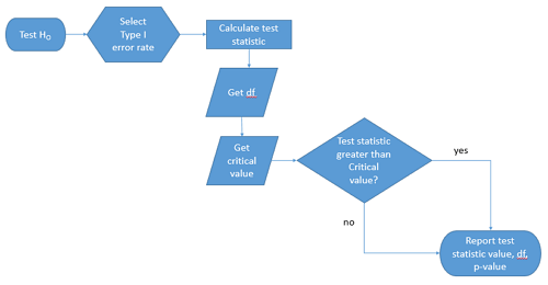
Figure 1. Flow chart of inductive statistical reasoning.
What’s missing from the flow chart is the very necessary caveat that interpretation of the null hypothesis is associated with two kinds of error, Type I error and Type II error. These points and others are discussed in the following sections.
We start with the hypothesis statements. For illustration we discuss hypotheses in terms of comparisons involving just two groups, also called two sample tests. One sample tests in contrast refer to scenarios where you compare a sample statistic to a population value. Extending these concepts to more than two samples is straightforward, but we leave that discussion to Chapters 12 – 18.
Null hypothesis
By far the most common application of the null hypothesis testing paradigm involves the comparisons of different treatment groups on some outcome variable. These kinds of null hypotheses are the subject of Chapters 8 through 12.
The Null hypothesis (HO) is a statement about the comparisons, eg, between a sample statistic and the population, or between two treatment groups. The former is referred to as a one tailed test whereas the latter is called a two-tailed test. The null hypothesis is typically “no statistical difference” between the comparisons.
For example, a one sample, two tailed null hypothesis.

and we read it as “there is no statistical difference between our sample mean and the population mean.” For the more likely case in which no population mean is available, we provide another example, a two sample, two tailed null hypothesis.

Here, we read the statement as “there is no difference between our two sample means.” Equivalently, we interpret the statement as both sample means estimate the same population mean.

Under the Neyman-Pearson approach to inference we have two hypotheses: the null hypothesis and the alternative hypothesis. The hull hypothesis was defined above.
Note 2: Tails of a test are discussed further in chapter 8.4.
Alternative hypothesis
Alternative hypothesis (HA): If we conclude that the null hypothesis is false, or rather and more precisely, we find that we provisionally fail to reject the null hypothesis, then we provisionally accept the alternative hypothesis. The view then is that something other than random chance has influenced the sample observations. Note that the pairing of null and alternative hypotheses covers all possible outcomes. We do not, however, say that we have evidence for the alternative hypothesis under this statistical regimen (Abelson 1995). We tested the null hypothesis, not the alternative hypothesis. Thus, it is incorrect to write that, having found a statistical difference between two drug treatments, say aspirin and acetaminophen for relief of migraine symptoms, it is not correct to conclude that we have proven the case that acetaminophen improves improves symptoms of migraine sufferers.
For the one sample, two tailed null hypothesis, the alternative hypothesis is

and we read it as “there is a statistical difference between our sample mean and the population mean.” For the two sample, two tailed null hypothesis, the alternative hypothesis would be

and we read it as “there is a statistical difference between our two sample means.”
Alternative hypothesis often may be the research hypothesis.
It may be helpful to distinguish between technical hypotheses, scientific hypothesis, or the equality of different kinds of treatments. Tests of technical hypotheses include the testing of statistical assumptions like normality assumption (see Chapter 13.3) and homogeneity of variances (Chapter 13.4). The results of inferences about technical hypotheses are used by the statistician to justify selection of parametric statistical tests (Chapter 13). The testing of some scientific hypothesis like whether or not there is a positive link between lifespan and insulin-like growth factor levels in humans (Fontana et al 2008), like the link between lifespan and IGFs in other organisms (Holtzenberger et al 2003), can be further advanced by considering multiple hypotheses and a test of nested hypotheses and evaluated either in Bayesian or likelihood approaches (Chapter 16 and Chapter 17). The advantage of the Bayesian approach is that it returns evidence for or against this hypothesis: if the posterior probability is greater than the prior probability, we can we say that we have evidence for the hypothesis. This is very appealing — the challenge is that the prior probability is inherently subjective (Chapter 6.4), limited by the amount and quality of existing information pertaining to the hypothesis (Prelec 2004).
Note 3: In Bayesian statistics, hypotheses and their parameters are treated as random variables and we can assign them probabilities. The prior probability is your initial belief about the likelihood of an event before adding new data. The posterior probability is the updated probability after new data has been added. Thus, the posterior combines your prior belief with the new information (the likelihood).
In the frequentis approach, the null hypothesis is no difference (no effect); in the Bayesian context, we’d treat this as a point estimate of zero and have to assign it a probability. In the absence of empirical evidence, one option is to set the probability as 50%, equal prior odds. Use of the spike and slab prior is likely a better approach. There’s a lot of work on these points; I refer interested readers to Campbell and Gustafson (2024) for additional readings and discussion.
How to interpret the results of a statistical test.
Any number of statistical tests may be used to calculate the value of the test statistic. For example, a one sample t-test may be used to evaluate the difference between the sample mean and the population mean (Chapter 8.5) or the independent sample t-test may be used to evaluate the difference between means of the control group and the treatment group (Chapter 10). The test statistic is the particular value of the outcome of our evaluation of the hypothesis and it is associated with the p-value. In other words, given the assumption of a particular probability distribution, in this case the t-distribution, we can associate a probability, the p-value, that we observed the particular value of the test statistic and the null hypothesis is true in the reference population.
By convention, we determine statistical significance (Cox 1982; Whitley & Ball 2002) by assigning ahead of time a decision probability called the Type I error rate, often given the symbol α (alpha). The practice is to look up the critical value that corresponds to the outcome of the test with degrees of freedom like your experiment and at the Type I error rate that you selected. The Degrees of Freedom (DF, df, or sometimes noted by the symbol v), are the number of independent pieces of information available to you. Knowing the degrees of freedom is a crucial piece of information for making the correct tests. Each statistical test has a specific formula for obtaining the independent information available for the statistical test. We first were introduced to DF when we calculated the sample variance with the Bessel correction, n – 1, instead of dividing through by n. With the df in hand, the value of the test statistic is compared to the critical value for our null hypothesis. If the test statistic is smaller than the critical value, we fail to reject the null hypothesis. If, however, the test statistic is greater than the critical value, then we provisionally reject the null hypothesis. This critical value comes from a probability distribution appropriate for the kind of sampling and properties of the measurement we are using. In other words, the rejection criterion for the null hypothesis is set to a critical value, which corresponds to a known probability, the Type I error rate.
Before proceeding with yet another interpretation, and hopefully less technical discussion about test statistics and critical values, we need to discuss the two types of statistical errors. The Type I error rate is the statistical error assigned to the probability that we may reject a null hypothesis as a result of our evaluation of our data when in fact in the reference population, the null hypothesis is, in fact, true. In Biology we generally use Type I error α = 0.05 level of significance. We say that the probability of obtaining the observed value AND HO is true is 1 in 20 (5%) if α = 0.05. Put another way, we are willing to reject the Null Hypothesis when there is only a 5% chance that the observations could occur and the Null hypothesis is still true. Our test statistic is associated with the p-value; the critical value is associated with the Type I error rate. If and only if the test statistic value equals the critical value will the p-value equal the Type I error rate.
The second error type associated with hypothesis testing is, β, the Type II statistical error rate. This is the case where we accept or fail to reject a null hypothesis based on our data, but in the reference population, the situation is that indeed, the null hypothesis is actually false. We must also keep in mind that, as we evaluate the p-value relative to the magnitude of the Type I error rate, and if we reject the null hypothesis, we still do not say that we have evidence for the alternative hypothesis.
Thus, we end with a concept that may take you a while to come to terms with — there are four, not two possible outcomes of an experiment.
Outcomes of an experiment
What are the possible outcomes of a comparative experiment\? We have two treatments, one in which subjects are given a treatment and the other, subjects receive a placebo. Subjects are followed and an outcome is measured. We calculate the descriptive statistics aka summary statistics, means, standard deviations, and perhaps other statistics, and then ask whether there is a difference between the statistics for the groups. So, two possible outcomes of the experiment, correct\? If the treatment has no effect, then we would expect the two groups to have roughly the same values for means, etc., in other words, any difference between the groups is due to chance fluctuations in the measurements and not because of any systematic effect due to the treatment received. Conversely, then if there is a difference due to the treatment, we expect to see a large enough difference in the statistics so that we would notice the systematic effect due to the treatment.
Actually, there are four, not two, possible outcomes of an experiment, just as there were four and not two conclusions about the results of a clinical assay. The four possible outcomes of a test of a statistical null hypothesis are illustrated in Table 1.
Table 1. When conducting hypothesis testing, four outcomes are possible.
| HO in the population | |||
| True | False | ||
| Result of statistical test | Reject HO | Type I error with probability equal to
α (alpha) |
Correct decision, with probability equal to
1 – β (1 – beta) |
| Fail to reject the HO | Correct decision with probability equal to
1 – α (1 – alpha) |
Type II error with probability equal to
β (beta) |
|
In the actual population, a thing happens or it doesn’t. The null hypothesis is either true or it is not. But we don’t have access to the reference population, we don’t have a census. In other words, there is truth, but we don’t have access to the truth. We can weight, assigned as a probability or p-value, our decisions by how likely our results are given the assumption that the truth is indeed “no difference.”
If you recall, we’ve seen a table like Table 1 before in our discussion of conditional probability and risk analysis (Chapter 7.3). We made the point that statistical inference and the interpretation of clinical tests are similar (Browner and Newman 1987). From the perspective of ordering a diagnostic test, the proper null hypothesis would be the patient does not have the disease. For your review, here’s that table (Table 2).
Table 2. Interpretations of results of a diagnostic or clinical test.
| Does the person have the disease\? | |||
| Yes | No | ||
| Result of the diagnostic test |
Positive | sensitivity of the test (a) | False positive (b) |
| Negative | False negative (c) | specificity of the test (d) | |
Thus, a positive diagnostic test result is interpreted as rejecting the null hypothesis. If the person actually does not have the disease, then the positive diagnostic test is a false positive.
Questions
- Match the corresponding entries in the two tables. For example, which outcome from the inference/hypothesis table matches specificity of the test \?
- Find three sources on the web for definitions of the p-value. Write out these definitions in your notes and compare them.
- In your own words distinguish between the test statistic and the critical value.
- All of our discussions have been about testing the null hypothesis, about accepting or rejecting, provisionally, the null hypothesis.
- What are the p-values for -logP of 5, 6, 7, 8, 9, and 10 \? Complete the p-value -logP transform table.
- Instead of log10 transform, create a similar table but for negative natural log transform. Which is more convenient? Hint:
log(x, base=exp(1))
Quiz Chapter 8.1
The null and alternate hypothesis
Chapter 8 contents
6.9 – Chi-square distribution
Introduction
As noted earlier, the normal deviate or Z score can be viewed as randomly sampled from the standard normal distribution. The chi-square distribution describes the probability distribution of the squared standardized normal deviates with degrees of freedom, df, equal to the number of samples taken. (The number of independent pieces of information needed to calculate the estimate, see Ch. 8.) We will use the chi-square distribution to test statistical significance of categorical variables in goodness of fit tests and contingency table problems.
The equation of the chi-square is
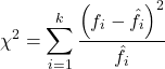
where k is the number of groups or categories, from 1 to k, and fi is the observed frequency and fi “hat” is the expected frequency for the kth category. We call the result of this calculation the chi-square test statistic. We evaluate how often that value or greater of a test statistic will occur by applying the chi-square distribution function. Graphs to show chi-square distribution for degrees of freedom equal to 1 – 5, 10, and 20 (Fig 1).
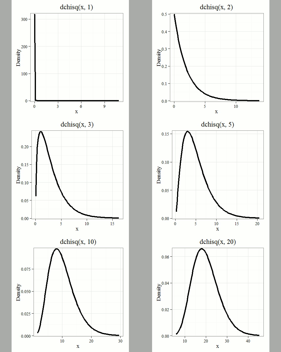
Figure 1. Animated GIF of plots of chi-square distribution over range of degrees of freedom.
Note that the distribution is asymmetric, particularly at low degrees of freedom. Thus tests using the chi-square are one-tailed (Fig 2).
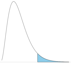
Figure 2. The test of the chi-square is typically one-tailed. In this case, probability of values greater than the critical value.
By convention in the Null Hypothesis Significance Testing protocol (NHST), we compare the test statistic to a critical value. The critical value is defined as the value of the test statistic — the cutoff boundary between statistical significance and insignificance — that occurs at the Type I error rate, which is typically set to 5%. The interpretation of the result is as follows: after calculating a test statistic, we can judge significance of the results relative to the null hypothesis expectation. If our test statistics is greater than the critical value, then the p-value of our results are less than 5% (R will report an exact p-value for the test statistic). You are not expected to be able to follow this logic just yet — rather, we teach it now as a sort of mechanical understanding to develop in the NHST tradition. The justification for this approach to testing of statistical significance is developed in Chapter 8. A portion of the critical values of the chi-square distribution are shown in Figure 3.
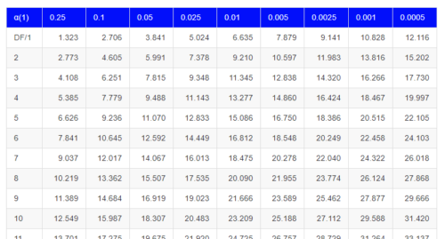
Figure 3. Portion of the table of some critical values of chi-square distribution, one tailed (right-tailed or “upper” portion of distribution).
See Appendix for a complete chi-square table.
The chi-squared test is a one-tailed test.
The result of the calculation of the test statistic is always non-negative because it is calculated by squaring the differences between the observed and expected frequencies. As a consequence, the test is always “right-tailed.”
The chi-square test does not provide information about the direction of an association, nor the strength of the association, only whether or not the variables are independent or associated. We use “correlation,” (eg, Phi coefficient or Cramer’s V, see Chapter 9.1 – Chi-square test: Goodness of fit and Chapter 9.2 – Chi-square contingency tables), to quantify the strength and direction of the association. While statistical significance is important, examining the direction and magnitude, the effect size, provides actionable insight and context for making informed decisions. For example, a new drug tested in a clinical trial may show an association between subject improvement (statistical significance), but yet have a small effect.
Example
Professor Hermon Bumpus of Brown University in Providence, Rhode Island, received 136 House Sparrows (Passer domesticus) after a severe winter storm 1 February 1898. The birds were collected from the ground; 72 of the birds survived, 64 did not (Table 1). Bumpus made several measures of morphology on the birds and the data set has served as a classical example of Natural Selection (Chicago Field Museum). We’ll look at this data set when we introduce Linear Regression.
Table 1. Survival statistics of Bumpus House sparrows
| Yes | No | |
| Female | 21 | 28 |
| Male | 51 | 36 |
Was there a survival difference between male and female House Sparrows? This is a classic contingency table analysis, something we will at length in Chapter 9. For now, we report the Chi-square test statistic for this test was 3.1264 and the test had one degree of freedom. What is the critical value of the chi-square distribution at 5% and one degree of freedom?. Typically we would simply use R to look this up
qchisq(c(0.05), df=1, lower.tail=FALSE)
But we can also get this from the table of critical values (Fig 4). Simply select the row based on the degrees of freedom for the test then scan to the column with the appropriate significance level, again, typically 5% (0.05).
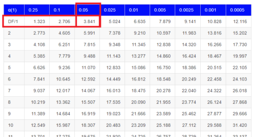
Figure 4. Portion of the chi-square distribution which shows how to find critical value of the chi-square distribution.
For 1 degree of freedom at 5% significance, the critical value is 3.841. Back to our hypothesis: Did male and female survival differ in the Bumpus data set? Following the NHST logic, if the test statistic value (eg, 3.1264) is greater than the critical value (3.841), then we would reject the null hypothesis. For this example, we would conclude no statistical difference between male and female survival because the test statistic was smaller than the critical value. How likely are these results due to chance? That’s where the p-value comes in. Our test statistic value falls between 5% and 10% (2.706 < 3.1264 < 3.841). In order to get the actual p-value of our test statistic we would need to use R.
R code
Given a chi-square test statistic you can use R to calculate the probability of that value against the null hypothesis. At the R prompt
pchisq(c(3.1264), df=1, lower.tail=FALSE)
And R output
[1] 0.07703368
Because we are using R Commander, simply select the command by following the menu options.
Rcmdr: Distributions → Continuous distributions → Chi-squared distribution → Chi-squared probabilities …
Enter the chi-square value and degrees of freedom (Fig 5).
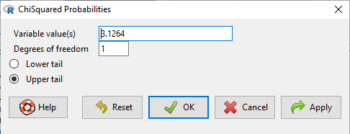
Figure 5. Screenshot of input box in Rcmdr for Chi-square probability values.
Questions
- What happens to the shape of the chi-square distribution as degrees of freedom are increased from 1 to 5 to 20 to 100?
Be able to answer these questions using the Chi-square table, Appendix 20.2, or using Rcmdr
- For probability α = 5%, what is the critical value of the chi-square distribution (upper tail)?
- The value of the chi-square test statistic is given as 12. With 3 degrees of freedom, what is the approximate probability of this value, or greater from the chi-square distribution?
Quiz Chapter 6.9
Chi-square distribution
Chapter 6 contents
- Introduction
- Some preliminaries
- Ratios and proportions
- Combinations and permutations
- Types of probability
- Discrete probability distributions
- Continuous distributions
- Normal distribution and the normal deviate (Z)
- Moments
- Chi-square (Χ2) distribution
- t distribution
- F distribution
- References and suggested readings
2.5 – Scientific method and where statistics fits
- Science isn’t just a recipe.
- Hypothetico-deductive reasoning.
- It’s all about the probability of a particular event.
- A statistical translation of the Scientific Method.
- When we say “experiment,” the hypothesis came first.
- Bottom-up, Top-down.
- How to interpret a test result.
- False discovery rate: claims must be stringently evaluated.
- Projects and the data lifecycle.
- Conclusions.
- Questions.
- Quiz.
- Chapter 2 contents .
Science isn’t just a recipe.
.
The scientific method is what makes science a “powerful way of knowing” (Church and Carpenter 2008), and by now, you should be familiar with the outline: hypothesis, experiment, etc. What distinguishes science from other fields of inquiry is that at its best, science accumulates verifiable evidence about our world. I begin with a disclaimer — our introductory textbooks tend to reify the scientific method (cf. Blachowicz 2009). Outside of the classroom and introductory science text books, I don’t think you’ll find much agreement among practicing scientists precisely what the scientific method entails, or whether strict adherence to a list of steps distinguishes what scientists do compared with other professions. For one difference, typical discussions of the scientific method may emphasize the experiment, which probably brings to mind images of a lab coat and test tubes, but should emphasize the critical thinking “tool kit” (Wivagg and Allchin 2002), eg, model-based inquiry. That said, holding a view that introductory textbooks should present nuances of epistemology seems a big ask.
But we do emphasize experimentation with good reason. In principle it is straightforward to identify what control groups are needed to conduct an experiment in the lab, but what are the control groups for an experiment conducted on the computer? In most cases, one should argue that if an outcome is obtained by random processes, then no additional cause need be addressed. Therefore, the control group for a simulation would be a random process generator.
Disagreements about the scientific method center about how science is really done (eg, from a social perspective), but also because there appear to be differences in approach in sciences that work on historical questions (physical cosmology, evolutionary biology, geology), and those that conform to the classic experimental approach (chemistry, molecular biology, physics). Epistemology is a fascinating area — How do we know what we know, What exactly is science and how is it different from other areas of knowing, etc. But I will leave you only with the tantalizing suggestion to read more and start with you with a list of readings to start (see Readings below). This is the stuff of graduate and professional school; we have work to do.
Despite apparent differences between what scientists say they do and how they actually do sciences, there is broad agreement; science as a way of knowing can be characterized by the following steps (National Academy of Sciences 1999).
- Begin with facts, which are observations confirmed and treated as true
- Formulate a hypothesis, with emphasis on hypotheses that are testable statements about relationships observed about the natural world
- Given the possible outcomes, state predictions derived from the hypothesis.
- Make observations of perform an experiment designed to test the hypothesis.
- Analyze the data from the experiment.
- Evaluate the results of the experiment against the predictions.
- Repeat.
This deceptively simple list hides much work to be done. Hypotheses are not “educated guesses,” where educated guess implies an idea about some phenomenon is likely the correct explanation because of the skill or knowledge of the person making the guess. Good hypotheses make possible experimental tests whose results can be used to rule out alternative explanations, sensu Platt’s “strong-inference”.
Hypothetico-deductive reasoning.
.
I mention this disclaimer about the common (and reassuring) textbook discourse on the scientific method to suggest that, if you have not already reached this point in your career, it is time to move past the cookbook approach to thinking about what it means to do science in practice. Yet another helpful reading is from a paper in Environmental Health by Ozonoff amd Grandjean (2020).
In other words, what makes “good science”?
There is induction and deduction and probabilistic thinking that must be grappled with, all emphasizing efforts by the individual, and yet science, if it is to make any progress must ultimately be a communal activity (Varmus 2009). In particular, to the extent a researcher consistently applies hypothetico-deductive reasoning, or as Platt (1964) called it, “strong-inference,” then good science can happen (see Fudge 2014 for an update). Strong inference according to Platt implies that researchers should follow three steps (after Fudge 2014):
- develop alternative hypotheses
- think of a crucial experiment that can exclude one or more hypotheses
- perform the experiment and obtain a clean result.
Then, beginning with step 1, repeat the procedure to refine the possibilities that remain.
The list of elements of the scientific method neglected to address the crucial role of scientists engaged in an active community of scientists fits in. However, we can can quickly suppose that every step of the scientific method can involve input from others to help shape, improve, and indeed carry out the activities needed to practice science. What scientists share is critical thinking and the tools of statistics provides a common language.
It’s all about the probability of a particular event.
.
Platt (1964) wrote that the observations we make that are puzzling or hard to explain, which implies our understanding is incomplete. We then proceed to ask questions about why the observations are different from our expectations, and we speculate about how the outcome comes about. Thus, we have to consider the probability, or chance, of a particular outcome (event) compare to other possible outcomes. Statistics is about analyzing the probability of outcomes. But there is a twist; there are two distinct, but complementary approaches to statistics. Most of the statistics you have been taught so far comes from the frequentist approach. That is, how often (frequency) will we get the kind of results we observe given the hypothesis? Another approach can be termed Bayesian, where the question is how likely is the hypothesis to be correct given the data? These two approaches view the data obtained from the same experiment differently. A frequentist views the data as random — repeat the experiment and the results will differ — but the hypothesis is fixed (it is either true or it is not). A Bayesian on the other hand views the hypothesis as random with a probability of being true somewhere between zero and 100 percent and the data are fixed.
Which are you, a frequentist, or a Bayesian? Consider the following from xkcd.com no. 1132 (Fig. 1).
Figure 1. “Frequentists vs Bayesians,” xkcd.com no. 1132
The Bayesian approach makes sense when there exists prior knowledge — the Sun came up this morning, as it did the day before, and the day before that, etc. New data are assessed against what we already know. The Frequentist approach, despite philosophical shortcomings, works for analyzing experiments where prior knowledge is lacking about outcomes. Because much of biomedical research is based on the Frequentist approach, most of our efforts, too, will utilize that approach.
A statistical translation of the Scientific Method.
.
Given our frequentist perspective, we can outline our Scientific Method as follows.
- Formulate a Null and an Alternative hypothesis.
- State predictions from the Null and an Alternative hypotheses.
- Design an experiment or observation.
- Analyze the data from the experiment or observation.
- Interpret the experiment or observation.
- Evaluate the predictions from the Null and an Alternative hypotheses.
- Accept (provisionally) or reject (provisionally) the Null hypothesis.
- Evaluate model fit and robustness
- Repeat.
In practice, there is more to statistics than these 8(9) steps, but this does provide the outline of what statistical analyses are about. There are nuances to how a Frequentist or a Bayesian views statistical analyses as evidence for or against a conclusion (Goodman 1999a, 1999b). We need to distinguish between when data are acquired in the process; data may come before or after the hypotheses are stated. In epistemology, hypotheses are either a priori or a posterori and we need to add these to our discussion of Scientific Method. The terms are Latin, translated apparently as “from the earlier” and “from the later, respectfully.
Note from the lists described as “the” scientific method how hypothesis comes first. Folks who think and write about how and why we know what we know — the discipline is called epistemology — tell us we are generally on more solid footing when we design experiments with specific intent, specific and testable hypotheses. The branch of statistics concerned with experimental design provides rich context for many practical aspects of how to implement experiments — in other words, how to follow the Scientific Method, even if turns out there isn’t just one universal definition of Scientific Methods out there.
When we say “experiment,” the hypothesis came first.
.
More commonly in statistics, the phrases planned, and therefore a priori, and unplanned or a posterori, comparisons are referenced. In practice, biologists design experiments and make observations accordingly to test one or more hypotheses, but they may also address additional hypotheses after the fact. Especially if the experiment generates a lot of data.
You may have also heard of the phrase data mining. Data mining is loosely defined, but mostly refers to sets of protocols and procedures to extract patterns from large data sets stored in databases. Google apparently does lots of data mining as do many other businesses that obtain large amounts of data. Unplanned comparisons includes any data mining protocols, no matter how sophisticated the language sounds (feature selection, classification tree). Data mining is not consistent with classic experiments; it’s different than Step 6 (Step 8 in the second list) listed above because no new data or experiment is carried out.
Can you get away with coming up with and testing new hypotheses from data gathered from an experiment designed to test a different hypothesis? Yes, and of course, the process can be quite profitable for Google. However, you should proceed with caution and restraint. If you are not careful about how you write it up — you will probably be called on it by a reviewer of your work. Is this a posterori approach still science? Of course, yes! I’d even go so far as to say that when one studies real systems, you can’t limit yourself to only planned hypotheses and testing. At least, one designs experiments and carries out those tests but then also uses current data to generate new ideas. Science is also exploratory — you may not design an experiment at all, but through observations, you probably will develop testable hypotheses! We’ll return to these concepts soon. What you must be aware of in any unplanned comparison or data mining sojourn is the possibility of committing a data dredging (aka p-hacking) sin — searching through data to come up with misleading, but statistically “significant” results (Ioannidis 2007; Stefan and Schönbrodt 2023).
Testing of unplanned a posterori hypotheses is a real concern in science. On the one hand, those who think about how we learn about the world and make sense of it have stated emphatically that the best way we know is to follow the scientific method — and that begins with hypotheses followed by designed experiments to test claims derived from those a priori hypotheses. We (teachers, textbook author) continue to teach science as the act of individuals toiling away in the forest or in the lab, pursuing sets of questions that may involve the collection of measurements on dozens to a few hundred subjects. While this type of science is still in practice, there is no doubt that big science involving many people is more common and, perhaps, better at generating new knowledge (Wuchty et al 2007). One result of “big science” is to generate a lot of data, the very essence now of big data, and there must be room for testing of new hypotheses gathered on data sets. This is the essence of the argument for the ENCODE project (ENCODE Project Consortium 2012) — generate lots of genetic data on the human genome using common techniques and make the data publicly available — new research can be conducted on old data.
Bottom-up, top-down.
.
Consider the pronouncements (almost daily it seems!) about the discovery of a new gene for some disease, process, or behavior in humans. Often times, although not always, these “discoveries” are not duplicated by other research groups. Why not? Well, for one, the phrase “gene for” is a dubious shorthand for what is usually a more complex causation. But from our statistical perspective it is problematic because the search for genes is really an a posterori exercise — one begins with phenotypic differences (some have the disease, others do not) and some genetic information (SNPs, DNA sequencing) and then proceeds to see if there are any differences in the genetic material at hand between the two groups. This approach, the Genome Wide Association Study, or GWAS, would be termed “top-down” — begin with the phenotypic differences and search for genetic differences between those that do and those who do not have the condition. Sampling is an issue (are the unaffected subjects a random sample from the entire population?), but the problem also is one of logical design — the hypothesis is made after the fact — a statistical difference between the groups is attributed to a particular genetic difference.
Case-control subjects, where patients with the condition are matched with other individuals who do not have the condition, but match in other ways (eg, age, income, etc.), are enrolled in such studies because there can be no random assignment of subjects to treatment. Case-control subjects are selected such that affected and unaffected individuals are matched by characteristics in as many meaningful ways as possible (eg, age, gender, income, etc.). Because many tests are conducted in GWAS studies, ie, is there a difference between the control and affected group for the first gene, the second gene, and so on up to the number of genes on the microarray chip (10,000 or more genes), the chance that any particular association is a false positive is high, discussed further when we cover Risk Analysis in Chapter 7.
How to interpret a test result.
You are a medical doctor reading the results of a test for three-month average glycated hemoglobin, A1C, levels for your patient. For example, A1C above 6% is considered strong marker of diabetes. A marker, yes, but not the same as a guarantee that a person has diabetes. A false positive (FP) is the case where a test result is positive, but the subject in fact does not have the condition. False positive is equal to the ratio of

where FP is number of false positive readings and TN refers to the true negative, those who in fact do not have the condition.
In Chapter 7 we will spend some time on risk analysis. To introduce this important subject in biostatistics, we’ll begin with an example. A study of 15,934 subjects without diagnosed diabetes found 3.8% or 605 individuals had elevated A1C levels, or about 7.1 million adults not yet diagnosed with diabetes (Selvin et al 2011). About 90% of these individuals also had fasting glucose levels greater than 100 mg/dL, i., diabetic. This is clearly a good test. However, note that 10% of the 605 individuals had elevated A1C, but fasting glucose levels less than 100 mg/dl, ie, did not meet the diagnostic of type 2 diabetes. Thus, the false positive rate is about 0.4%, or nearly 30,000 adults with elevated A1C without diabetes.
Working through frequencies can be challenging, so applying a natural number approach helps. Having just read through the frequencies and percentages, now look at how they translate to probability tree (Fig. 2). Start by utilizing a per capita rate standard: for proportions in the 10 – 20% range, a standard 1000 persons works well (Fig. 2).
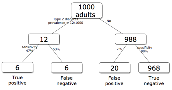
Figure 2. Probability tree diagram with prevalence of type 2 diabetes and sensitivity, specificity of A1C test, data from CDC and Selvin et al 2011. Tree drawn with free diagrams.net app.
How many expected to have A1C above 6%? Twenty-six total positives, only 23% are true positives. An important lesson is that if the prevalence of a condition is low, then any diagnostic test with high sensitivity necessarily will identify many false positives.
False discovery rate: claims must be stringently evaluated.
.
The genome scientists involved in GWAS studies generally are aware of false positives, also termed false discovery rate (FDR), conduct statistical corrections to account for false positives (eg, Brzyski et al 2016), and generally are cautious in their interpretation. But not always. Studies of associations between autism and environment come to mind (eg, Waldman et al 2008), and recent developments in the direct-to-consumer genetic testing market also suggest that the limitations of these kinds of studies are not always represented.
There is a broader concern about the reliability of research, and the debate about how to improve reliability comes from a call to understand how to do statistics better and, more importantly to understand how statistics are to be used in making claims from statistical results (Ioannidis 2007; but see Goodman and Greenland 2007). A key element of scientific work is that findings are repeatable: results from one group should apply to other groups. One dictate to improve reproducibility — increase number of subjects in studies — is obvious, but given the cost of GWAS, currently an unreasonable demand.
In some cases, biologists already have a particular gene in mind, whose function is more or less known, and then the exercise follows the Scientific Method listing much more directly. This bottom-up approach leads to a straightforward, testable genetic hypotheses: a specific difference in genomic sequence predicts a difference in phenotype outcome. A good example is the identification of more than 100 different single nucleotide mutations, called single nucleotide polymorphisms or SNPs, in the CFTR gene of patients known to have cystic fibrosis disease (Castellani 2013). As of August 2018, the number of known pathogenic or likely pathogenic SNPs is now listed at 440 in the SNP database; to put this in some context, there are more than 40,000 reported single nucleotide polymorphisms for the CFTR gene (this number includes SNP duplicates).
Projects and the data lifecycle.
A requirement for our biostatistics course, students are asked to design and implement a research project during the semester (Hydorn 2019). The project can either be part of an ongoing student research project or solely confined to the biostatistics course. The topics are diverse, ranging from observational to experimental to systematic reviews from the disciplines of biology, environmental science, and public health. Examples of project ideas implemented in the biostatistics and related courses at Chaminade University include:
- effects of environmental stress on growth rates.
- 2D and 3D shape analysis of mollusk shells.
- Individual variation and fluctuating asymmetry of plant leaves and flowers along an altitudinal gradient
- several systematic reviews (meta analysis) of published works of interest to public health
- vaccination benefits and risks.
- pain management of over the counter vs prescription medication.
- efficacy of “alternative medicine” approaches to health.
- comparisons of types of medical insurance on patient outcomes of knee replacement therapy.
The justification for the project learning activity is that it provides hands-on opportunity to apply statistical and data sciences concepts to real-world problems. Students work through the challenges of developing a research question, identifying testable hypotheses, designing a study, collecting data, performing analysis, and interpreting results. Importantly, students must decide for themselves which statistical tests and methods are most appropriate for their unique data, rather than simply following a formula presented in a lecture. This connects abstract statistical ideas to practical application, promoting a deeper, more lasting understanding. We manage the projects by encouraging a research lab community: students discuss with their peers their ideas, their data collection and experimental design challenges, with the instructor serving to guide and mentor the multiple projects and intervene as needed to steer student projects towards completion.
Throughout the semester we model the project approach. Students are encouraged to create a working folder on their computer, while dividing homework and other assignments into named projects. Students are also asked to address aspects of their project’s data life cycle (Borgman 2019, Ezer and Whitacker 2019, Griffin et al 2018). A quick Google search on the phrase returns millions of hits (see Note 1), but key elements of the concept are that projects have a beginning and an end, and it is helpful — and in the case of our statistics course, required — to address project management.
Note 1: For example, “8 Steps in the Data Life Cycle,” by Tim Tobierski of Harvard Business School.
BI-311 students, see Homework 1: Project data life cycle in Mike’s Workbook for Biostatistics.
Projects include data generation and collection, data processing, storage and data management, data exploration and visualization, interpretation and reporting. Thus, students need to develop a data management plan, which includes how data are collected, application of best practices to insure data file and storage of images, and how to share the project results. We ask students to develop 10-min research talks, which are presented and recorded, suitable for ePortfolio inclusion.
Conclusions.
.
Epistemology, the theory of how knowledge is acquired, is a complicated business – what I want you to appreciate now is that planned and unplanned comparisons affect interpretation of your statistical results, how the difference is likely also to affect the reproducibility of your work. In the language or clinical trials and experimental design, planned and unplanned accompany prospective and retrospective studies (Chapter 5). A prospective study in the case of GWAS means genetic differences among individuals are known at the start of the study, and phenotypic differences arise naturally during the course of the study. Knowing the strengths and limitations of, for example, a planned retrospective study is at the heart of experimental design (Chapter 5).
In the biostatistics course, students are required to design and carry out an independent research project that integrates statistical methods with real-world problems in biology, environmental science, or public health. The course emphasizes hands-on learning through the full research process—from formulating questions to data collection, analysis, and interpretation—while fostering a collaborative research lab environment. Students also learn project and data management skills and conclude by presenting their findings in recorded research talks suitable for inclusion in an ePortfolio.
Questions.
- Write up three learning outcomes for this page. Hint: Point your favorite generative AI to this page and ask for help.
- Above we described how GWAS studies are generally top-down; What would constitute a bottom-up approach to GWAS?
- In your own words provide pro and con points of view on data mining of large data sets.
- Create a stylized infographic, like a mind map, to illustrate the data life cycle for a one semester research project.
Quiz Chapter 2.5
Scientific method and where statistics fits
Chapter 2 contents
.