5.3 – Replication, Bias, and Nuisance Variables
Introduction
This page describes additional elements of experimental design, replication and bias, which can impact the validity of a study.
Replication in science refers to repeating an experiment under identical conditions multiple times. To the extent the same conclusions are achieved, we can say the outcome is reproducible (Simmons 2014) and, therefore, likely to be objectively true (Earp 2011). Replication of experimental and sampling units is an essential component of good experimental design. Confusing technical replicates for biological replicates is called pseudoreplication.
Bias refers to any of a number of sociological and cognitive errors which may influence conclusions in science (Ionnidis 2005). In a meta-analysis, Fanelli et al (2017) reported that while the size of effect from identifiable biases were small, some disciplines were more prone to these sources of error. That researchers testing similar hypotheses reach different conclusions may result from bias. One such bias is positive outcome bias, where reports of null hypotheses are more often rejected than they should be based on sample size and other concerns of statistical power (see Chapter 11 – Power analysis).
The page concludes with a discussion of nuisance variables, variables that may be causally associated with the outcome of interest, but themselves are either of no interest in the study, or may not be known in advance (Meehl 1970; see also discussion of spurious correlations in Chapter 16.3 – Data aggregation and correlation).
Technical vs. biological replicates.
A laboratory technician retrieves a vial of an immortalized cell line from cryostorage and initiate propagation of the cells for the week’s work. After a couple of days of subculturing, the technician has grown millions of cells and is ready to set up an assay. After washing the cells in PBS (phosphate buffered saline), the technician adjusts the concentration of cells to 10,000 per mL media, places the tube on ice, and proceeds to set up a 48 well microplate. To each well, the technician adds media, one or more agents (Table 1), plus cells, total volume each well at one mL, three replicates per treatment.
Table 1. In our example there were four treatments plus a control (media only)
- DMSO only (D)
- DMSO + Cytokine (DC)
- DMSO + Small molecule Inhibitor (DS)
- DMSO + Cytokine + Small molecule Inhibitor (DCS)
- Media only (M)
The plate table might look something like Figure 1.

Figure 1. Schematics of a set up for a hypothetical 48 well microplate (plate_plot() from ggplate package).
The technician has done a lot of work; but, from a statistician’s point of view, effectively the technician has but one sampling unit to show for his efforts; one biological sampling unit because as far as we can tell, the cells were all related. Biological replication refers to repeat measures (eg, same conditions) on biologically distinct entities (Blainey et al 2014). Technical replication, in contrast, refers to repeat measures on the same entity, eg, the same individual (Blainey et al 2014).
However, there were more than one technical samples in the experimental design, twelve in all because there were twelve wells. Many of you will recognize this as the distinction between technical and biological replicates. In thinking about experimental design replicates pertain to the number of sampling units that are treated the same way. In our example cells may be “treated the same way” in at least two distinct ways. Biologically, the cells may be the same: derived from the same clonal cell, all at the same passage (generation) number, each cell genetically, morphologically, physiologically (etc.,) identical to the next cell. Technical replication on the other hand pertains to the levels of the treatments.
Within each of these treatments we had three wells, and that’s at the level of the technical replication.
A final note on this experiment. We as molecular biologists call each of these treatment groups, but statisticians thinking of this design would recognize only one treatment (called in statistics a factor), with four levels of the treatment. We will discuss this beginning in chapter 12 when we introduce analysis of variance.
Types of bias.
When we make decisions, we like to think we are rational; that we make decisions based on an evaluation of evidence. And yet, an increasing body of literature suggests that our decisions often made in a manner that falls short of rational processing. We outlined some sources of bias in Chapter 2.6. Deviance from rational decision making is due to any number of cognitive biases we may have. Researchers and medical doctors make many decisions and, unfortunately, are just as susceptible to cognitive biases as the rest of us. One kind of bias that is bedeviling to research is confirmatory bias. Confirmatory bias refers to a researcher in effect seeking evidence in a way that confirms a prior conclusion (Kaptchuck 2003). Confirmatory bias would be exhibited if we report positive effects of aspirin to relieve migraines in subjects, but exclude cases where the subjects report no improvement. Medical doctors may be risk averse and therefore tend to over-prescribe, or they may be risk-takers (eg, rise and fall of high-dose chemotherapy, cf, discussion in Howard et al. 2011).
The concept of bias was first introduced in Chapter 3 and will be returned to in subsequent chapters. In general, bias refers to the objectivity of measurement and inferences about such measurements. Bias implies that a series of measurements consistently fail to return the true value of the variable. Bias is systematic error and may be associated with a poorly calibrated instrument or even the use of improper sets of rules for measurement given the nature of the characteristic. Bias can be captured by the concept of accuracy.
Bias is challenging to eliminate; the best way is to design the experiment so that the observer, the researcher, is unaware of the specific questions to be tested. The research is conducted “blind.” Clinical research provides the easiest examples. A trial can be blind in a couple of ways:
- The subjects do not know which treatment they receive, but the researcher does know
- The researcher does not know which treatment subjects receive, but the subjects know
- Neither the researcher nor the subjects know which treatment they receive.
- The other possibility is that both the researcher and the subjects know treatments received — this would be a poor design.
Bias can enter a research project at multiple levels. A partial list of sources of bias in research includes (modified after Pannucci and Wikins 2010):
Bias that occurs before the experiment
- Inadequate planning of the experiment, flawed design
- Bias in selection of subjects from the reference population
- Surveillance bias, where one group is studied more closely than another group.
Surveillance bias, also called detection bias or ascertainment bias, a type of information bias. Characterized as “the more you look, the more you find (Sackett 1979),” differences in outcome counts varies with differences in effort to detect. Recently, cases of myocarditis in young people were reported following Covid-19 mRNA vaccination (eg, Bozkurt et al 2021. Marshall et al 2021). However, myocarditis reports following vaccination occur at the rates expected in the population, and the reports lack important context (eg, other respiratory viruses known to cause myocarditis not ruled out), suggesting the putative link between Covid-19 vaccines and this heart condition may be result of us looking hard for signs of adverse effects of the vaccine (cf, discussion in O’Leary and Maldonado 2021).
Bias during the experiment
- Interviewer bias
- Chronology bias
- Recall bias
- Transfer bias
- Misclassification of exposure or outcome
- Performance bias
Performance bias refers to conditions of an experiment that introduce unintended differences between groups. For example, subjects enrolled in a weight-loss study randomly assigned to the control group may react poorly when they realize they are not receiving the experimental intervention. This leads to potential for a systematic bias — participants in the control group may behave differently, counteracting the point of randomization (McCambridge et al 2014).
Another well-known performance bias is associated with eliciting maximal performance from animals, such as running stamina or maximum sprint running speed (Losos et al 2002). For example, spring running speed of lizards may be measured by placing lizards onto a high-speed treadmill, then increasing belt speed to match the individual’s burst performance (eg, Dohm et al 1998). Clearly, not all individuals will perform to maximum physiological capabilities under these conditions.
Bias after the experiment
- Citation bias
- Confounding
Another way to view sources of bias is that, at least from the perspective of the researcher, the bias is likely to be unconscious bias. After all, if we knew about the sources of bias we would work our experiments in such a way to minimize known error producing sources (Holman et al 2015). Selecting subjects at random and keeping record keeping blind with respect to treatments are among the best tools we have to avoid this kind of bias.
Nuisance variables
A key quality of experimental design is the opportunity afforded the researcher to apply control. In a classic view of the experiment, one allows only one aspect to vary, the treatment applied, all else is controlled. Thus, any difference in outcome may be attributed to the treatment. However, it is likely impossible to control for all possible variables that may affect our outcome; confounding clear interpretation of results (see Chapter 16.2 and 16.3). Consider, for example, the effects of age on running performance (Fig. 2).
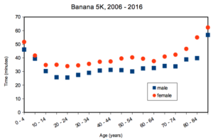
Figure 2. Mean 5K running times (minutes) by age and gender (2006 – 2016, Jamba Juice Banana 5K race, Honolulu, HI).
If we are interested in gender differences, we must also deal with the change in performance with age: older runners regardless of gender tend to run slower than younger runners. Thus, in the comparison of genders, age is a nuisance variable. In the literature, you may see “lurking variable,” or other such names. The concept is that these variables may be causal, but are either of no interest in the study, or may not be known in advance. Therefore, age must be accounted for before we can address gender differences, if any. Age, in this case, is considered a nuisance variable because we are not primarily interested in age effects, but age clearly covaries (is associated) with running performance. How best to handle nuisance variables? One approach is to match by age (blocking effect, see Chapter 14.4); another approach would be to randomly select with respect to age when compiling female and male times.
Another example of confounding. Results from ecological experiments intended to test for presence of competition for resources by plant species by removing plants may alter herbivory levels; thus, survivorship not the result of reduced plant-plant competition but because of changes in herbivore behavior (Reader 1992).
Questions
- I cite a number of articles in Mike’s Biostatistics Book. If you’re paying attention, you’ll have noticed that all of my citations, at least for articles, link to a source that you can either download or read online. What kind of error am I committing by following this approach?
- In large part because of the tendency for overuse of antibiotics, doctors are less likely today to prescribe antibiotics for patients with upper respiratory tract infections than in the past (Zoorob et al 2012). URTI are mostly caused by rhinovirus infections (Calderaro et al 2022) and, therefore, the course of infection in a patient should be unaffected by addition of antibiotic. However, although rare compared to URTI, life-threatening illness like acute epiglottitis caused by bacteria infection can sometimes develop or accompany URTI. Thus, not prescribing antibiotics at a diagnosis of URTI may risk a worsening condition for the patients. This sets the doctor up for a potential cognitive bias – to prescribe or not to prescribe antibiotics prophylactically? Discuss this decision in the context of potential sources of cognitive biases and possible outcomes of the decision.
Quiz Chapter 5.3
Replication, bias, and nuisance variables
Chapter 5 contents
- The basics explained
- Experiments
- Experimental and Sampling units
- Replication, Bias, and Nuisance Variables
- Clinical trials
- Importance of randomization in experimental design
- Sampling from Populations
- References and suggested readings
5.2 – Experimental units, Sampling units
Introduction.
Sampling units refer to the measured items, the focus of data collection; samples are selected from populations. Often, sampling units are the same thing as individuals. For example, if we are interested in the knowing whether men are more obese than women in Hawai’i, we would select individuals from the population; we would measure individuals. Thus, the sampling unit would be individuals, and the measurement unit would be percent body fat recorded for each individual. The data set would be the collection of all body fat measures for all individuals in the study, and we would then make inferences (draw conclusions) about the differences, if any, between adult males and females for body fat.
But sampling units can also refer to something more restrictive than the individual. For example, we may be interested in how stable, or consistent, is a person’s body fat over time. If we take a body fat measure once per year over a decade on the same group of adults, then the sampling unit refers to each observation of body fat recorded (once per year, ten times for an individual), and the population we are most likely to be referring to is the collection of all such readings (ten is arbitrary — we could have potentially measured the same individual thousands of times).
In some cases the researcher may wish to compare groups of individuals and not the individuals themselves. For example, a 2001 study sought to see if family structure influenced the metabolic (glycemic) control of children with diabetes (Thompson et al 2001). The researchers compared how well metabolic control was achieved in children of single parents and two-parent families. Thus, the sampling units would be families and not the individual children.
Experimental units.
Experimental units refers to the level at which treatments are independently applied in a study. Often, but not always, treatments are applied directly to individuals and therefore the sampling units and experimental units in these cases would be the same.
Question 1: What is the sampling unit in the following cell experiment?
A technician thaws a cryo tube containing about ½ million A549 cells (Foster et al 1998) and grows the cells in a T-75 culture flask (the 75 corresponds to 75 cm2 growing area) in a CO2 incubator at 37 °C. After the cells reach about 70% confluency, which may represent hundreds of thousands of cells, the technician aliquots 1000 cells into twelve wells of a plate for a total of 12000 cells. To three wells the technician adds a cytokine, to another three wells he adds a cytokine inhibitor, and to another three wells he adds both the cytokine and it’s inhibitor, and to the last three wells he adds DMSO, which was the solvent for both the cytokine and the inhibitor. He then returns the plate to the incubator and 24 hours later extracts all of the cells and performs a multiplex quantitative PCR to determine gene expression of several target genes known to be relevant to cell proliferation.
The described experiment would be an example of a routine, but not trivial procedure the technician would do in the course of working on the project in a molecular biology laboratory.
The choices for numbers provided in the description we may consider for the number of sampling units are:
- 1000 cells
- 12,000 cells
- ½ million cells
- 3 wells
- 12 wells
- The target genes
- None of the above
The correct answer is G, None of the above.
“None of the above” because the correct answer is … there was just one sampling unit! All cells trace back to that single cryo tube.
To answer the question, start from the end and work your way back. What we are looking for is independence of samples and at what level in the experiment we find independence. Our basic choice is between numbers of cells and numbers of wells. Clearly, cells are contained in the wells, so all of the cells in one well share the same medium, being treated the same way, including all the way back to the cryo tube — all of the cells came from that one tube so this lack of independence traces all the way back to the source of the cells. Thus, the answer can’t be related to cell number. How many wells did the technician set up? Twelve total. So, the maximum number of sampling units would be twelve, unless the samples are not independent. And clearly the wells (samples) are not independent because, again, all cells in the twelve wells trace back to a single cryo tube. Thus, from both perspectives, wells and cells, the answer is actually just one sampling unit! (Cumming et al 2007; Lazic 2010). Finally, the genes themselves are the targets of our study — they are the variables, not the samples. Moreover, the same logic applies — all copies of the genes are in effect descended from the few cells used to start the population.
Experimental and sampling units often, but not always the same.
Question 2: What is the experimental unit in the described cell experiment?
- 1000 cells
- 12,000 cells
- ½ million cells
- 3 wells
- 12 wells
- The target genes
- None of the above
The correct answer is E, 12 wells. Noted above, the technician applied treatments to 12 wells. DMSO was added to all wells. There were three treatments, cytokine, inhibitor, and cytokine-inhibitor (Table 1).
Table 1. Translate experiment description to a table to better visualize the design
| Wells | Treatment |
|---|---|
| A1 | Cytokine |
| A2 | Cytokine |
| A3 | Cytokine |
| A4 | DMSO |
| B1 | Inhibitor |
| B2 | Inhibitor |
| B3 | Inhibitor |
| B4 | DMSO |
| C1 | Cytokine+Inhibitor |
| C2 | Cytokine+Inhibitor |
| C4 | Cytokine+Inhibitor |
| C4 | DMSO |
Note 1: Use package ggplate to create a simple graphic to visualize a culture plate.
table01.ch05.2 <- data.frame(
     well = c("A1", "A2", "A3", "B1", "B2", "B3", "C1",
              "C2", "C3", "A4", "B4", "C4", "D4"),
     treatment = c(rep("Cytokine", 3), rep("Inhibitor", 3),
              rep("Cytokine + Inhibitor", 3), rep("DMSO", 4))
     )
plate_plot(data = table01.ch05.2,
     position = Well,
     value = Treatment,
     plate_size = 12,
     plate_type = "round")
which results in this nice plate layout (Fig 1)

Figure 1. Plate layout for Table 1. Plot made with plate_plot() function from R package ggplate.
If observations were made, then the same function can display values. Add a column of values to the dataset (eg, “Values”), then add another value = line, eg, value = Values to the R code.
Replication: Groups and individuals as sampling units.
The correct identification of levels at which sampling independence occurs is crucial to successful interpretation of inferential statistics.
Note 2:replication in Table 1: three cytokine, three cytokine-inhibitor, three with both.
Sampling error rate is evaluated at the level of the sampling units. Technical replication of sampling units allows one to evaluate errors of measurement (eg, instrument noise) (Blainey et al 2014) and other sources of technical sources of noise.
Note 3: Data noise refers to random or irrelevant information that corrupts the “true” signal in a dataset, introducing variability and potential errors. A nuisance variable is a specific type of noise that is fundamental to the data collection process but not of interest to the researcher, and its effect must be accounted for or removed via pre-processing steps. For approaches to control for noise, see Chapter 17.4 and Chapter 20.3 for more.
Replication of sampling units increases statistical power, the ability to correctly reject hypotheses. If the correct design reflects sampling units are groups and not individuals, then by counting the individuals as the independent sampling units would lead the researcher to think his design has more replication than it actually does. The consequence on the inferential statistics is that he will more likely reject a correct null hypothesis, in other words, the risk of elevated type I error occurs (Chapter 8 – Inferential statistics). This error, confusing individual and group sampling units, is called pseudoreplication (Lazic 2010).
Consider a simpler experimental design scenario depicted in Figure 2: Three different water treatments (eg, concentrations of synthetic progestins, Zeilinger et al. 2009) in bowls A, B, and C; three fish in bowl A, three fish in bowl B, and three fish in bowl C. The outcome variable might be a stress indicator, eg, plasma cortisol (Luz et al 2008).
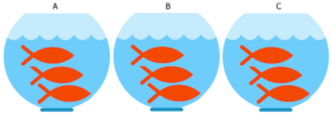
Figure 2. Three aquariums, three fish. Image modified from https://www.pngrepo.com/svg/153528/aquarium
Question 3: What were the experimental units for the fish in the bowl experiment (Fig 2)?
- Three bowls
- Nine fish
- Three water treatments
The correct answer is A, 3 bowls. The treatments were allocated to the bowls, not to individual fish. The three fish in each bowl provides technical replication for the effects of bowl A, bowl B, and bowl C, but does not provide replication for the effects of the water treatments. Adding three bowls for each water treatment, each with three fish, would be the simplest correction of the design, but may not be available to the researcher because of space or cost limitations. The design would then include nine bowls and 27 fish. If resources are not available to simply scale up the design, then the researcher could repeat the study several times, taking care to control nuisance variables (Chapter 5.3). Alternatively, if the treatments were applied to the individual fish, then the experimental units become the individual fish and the bowls reduced to a blocking effect (Chapter 14.4), where differences may exist among the bowls, but they are no longer the level by which measurements are made.
Note 4: If pseudoreplication is present in a study, then this may be accounted for by specifying the error structure in a linear mixed model (eg, random effects, blocking effects, etc., see Chapter 14 and Chapter 18).
Question 4: What were the sampling units for the fish in the bowl experiment (Fig 2)?
- Three bowls
- Nine fish
- Three water treatments
The correct answer is B, the individual fish. If instead of aqueous application of synthetic progestin, treatments were applied directly to each fish via injection, what would be the answers to Question 3 and Question 4?
Choices like these clearly involve additional compromises and assumptions about experimental design and inference about hypotheses.
Conclusion.
Sampling units, experimental units, and the concept of level at which units are independent within an experiment were introduced. Lack of independence yields the problem of pseudoreplication in an experiment, which will increase the chance that we will detect differences between our treatment groups, when no such difference exists!
Questions.

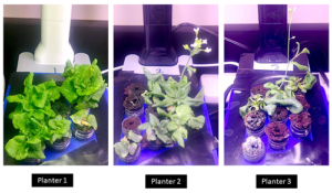
Figure 3. Three Miracle-Gro AeroGarden planters®, each with nine seedlings of an Arabidopsis thaliana strain.
Nine seeds each of three strains of Arabidopsis thaliana were germinated in three Miracle-Grow AeroGarden® hydroponic planters (Fig 3). Each planter had nine or ten vials with sphagnum peat. All seeds from a strain were planted in the same apparatus, one seed per vial. With respect to this experimental design
1. Define experimental units and sampling units.
2. Provide design examples where the experimental units are the same as the sampling units.
3. With respect to the independent and dependent (outcome) variables, discuss impacts of nuisance variables.
Quiz Chapter 5.2
Experimental units, Sampling units