17.8 – Assumptions and model diagnostics for Simple Linear Regression
Introduction
The assumptions for all linear regression:
- Linear model is appropriate.
The data are well described (fit) by a linear model. - Independent values of Y and equal variances.
Although there can be more than one Y for any value of X, the Y‘s cannot be related to each other (that’s what we mean by independent). Since we allow for multiple Y‘s for each X, then we assume that the variances of the range of Y‘s are equal for each X value (this is similar to our ANOVA assumptions for equal variance by groups). Another term for equal variances is homoscedasticity. - Normality.
For each X value there is a normal distribution of Y‘s (think of doing the experiment over and over). - Error
The residuals (error) are normally distributed with a mean of zero.
Note 1
Note the mnemonic device: Linear, Independent, Normal, Error or LINE.
Each of the four elements will be discussed below in the context of Model Diagnostics. These assumptions apply to how the model fits the data. There are other assumptions that, if violated, imply you should use a different method for estimating the parameters of the model.
Ordinary least squares makes the additional assumption about the quality of the independent variable that e that measurement of X is done without error. Measurement error is a fact of life in science, but the influence of error on regression differs if the error is associated with the dependent or independent variable. Measurement error in the dependent variable increases the dispersion of the residuals but will not affect the estimates of the coefficients; error associated with the independent variables, however, will affect estimates of the slope. In short, error in X leads to biased estimates of the slope.
The equivalent, but less restrictive practical application of this assumption is that the error in X is at least negligible compared to the measurements in the dependent variable.
Multiple regression makes one more assumption, about the relationship between the predictor variables (the X variables). The assumption is that there is no multicollinearity, a subject we will bring up next time (see Chapter 18).
Model diagnostics
We just reviewed how to evaluate the estimates of the coefficients of the model. Now we need to address a deeper meaning — how well the model explains the data. Consider a simple linear regression first. If Ho: b = 0 is not rejected — then the slope of the regression equation is taken to not differ from zero. We would conclude that if repeated samples were drawn from the population, on average, the regression equation would not fit the data well (lots of scatter) and it would not yield useful prediction.
However, recall that we assume that the fit is linear. One assumption we make in regression is that a line can, in fact, be used to describe the relationship between X and Y.
Here are two very different situations where the slope = 0.
Example 1. Linear Slope = 0, No relationship between X and Y
Example 2. Linear Slope = 0, A significant relationship between X and Y
But even if Ho: b = 0 is rejected (and we conclude that a linear relationship between X and Y is present), we still need to be concerned about the fit of the line to the data — the relationship may be more nonlinear than linear, for example. Here are two very different situations where the slope is not equal to 0.
Example 3. Linear Slope > 0, a linear relationship between X and Y
Example 4. Linear Slope > 0, curve-linear relationship between X and Y
How can you tell the difference? There are many regression diagnostic tests, many more than we can cover, but you can start with looking at the coefficient of determination (low R2 means low fit to the line), and we can look at the pattern of residuals plotted against the either the predicted values or the X variables (my favorite). The important points are:
- In linear regression, you fit a model (the slope + intercept) to the data;
- We want the usual hypothesis tests (are the coefficients different from zero?) and
- We need to check to see if the model fits the data well. Just like in our discussions of chi-square, a “perfect fit would mean that the difference between our model and the data would be zero.
Graph options
Using residual plots to diagnose regression equations
Yes, we need to test the coefficients (intercept Ho = 0; slope Ho = 0) of a regression equation, but we also must decide if a regression is an appropriate description of the data. This topic includes the use of diagnostic tests in regression. We address this question chiefly by looking at
- scatterplots of the independent (predictor) variable(s) vs. dependent (response) variable(s).
what patterns appear between X and Y? Do your eyes tell you “Line”? “Curve”? “No relation”? - coefficient of determination
closer to zero than to one? - patterns of residuals plotted against the X variables (other types of residual plots are used to, this is one of my favorites)
Our approach is to utilize graphics along with statistical tests designed to address the assumptions.
One typical choice is to see if there are patterns in the residual values plotted against the predictor variable. If the LINE assumptions hold for your data set, then the residuals should have a mean of zero with scatter about the mean. Deviations from LINE assumptions will show up in residual plots.
Here are examples of POSSIBLE outcomes:
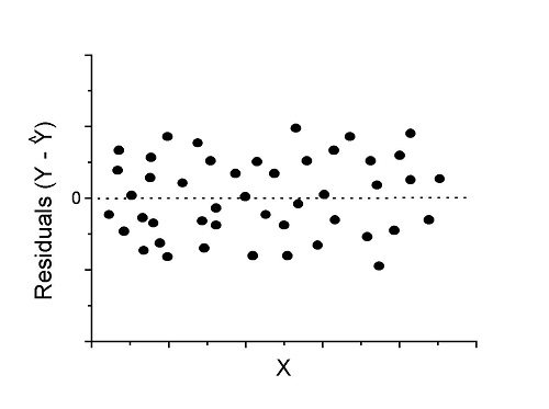
Figure 1. An ideal plot of residuals
Solution: Proceed! Assumptions of linear regression met.
Compare to plots of residuals that differ from the ideal.
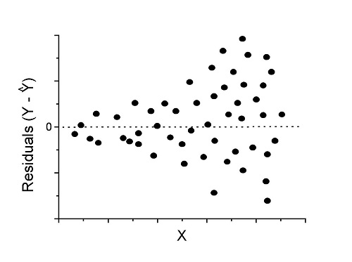
Figure 2. We have a problem. Residual plot shows a “funnel” shape — unequal variance (aka heteroscedasticity).
Solution. Try a transform like the log10-transform.
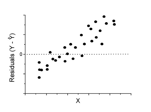
Figure 3. Problem. Residual plot shows systematic trend.
Solution. Linear model a poor fit; May be related to measurement errors for one or more predictor variables. Try adding an additional predictor variable or model the error in your general linear model.
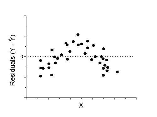
Figure 4. Problem. Residual plot shows nonlinear trend.
Solution. Transform data or use more complex model
This is a good time to mention that in statistical analyses, one often needs to do multiple rounds of analyses, involving description and plots, tests of assumptions, tests of inference. With regression, in particular, we also need to decide if our model (e.g., linear equation) is a good description of the data.
Diagnostic plot examples
Return to our example.Tadpole dataset. To obtain residual plots, Rcmdr: Models → Graphs → Basic diagnostic plots yields four graphs. Graph A is
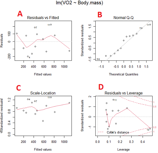
Figure 5. Basic diagnostic plots. A: residual plot; B: Q-Q plot of residuals; C: Scale-location (aka spread-location) plot; D: leverage residual plot.
In brief, we look at plots
A, the residual plot, to see if there are trends in the residuals. We are looking for a spread of points equally above and below the mean of zero. In Figure 5 we count seven points above and six points below zero so there’s no indication of a trend in the residuals vs the fitted VO2 (Y) values.
B, the Q-Q plot is used to see if normality holds. As discussed before, if our data are more or less normally distributed, then points will fall along a straight line in a Q-Q plot.
C, the Scale- or spread-location plot is used to verify equal variances of errors.
D, Leverage plot — looks to see if an outlier has leverage on the fit of the line to the data, i.e., changes the slope. Additionally, provides location of Cook’s distance measure (dashed red lines). Cook’s distance measures the effect on the regression by removing one point at a time and then fitting a line to the data. Points outside the dashed lines have influence.
A note of caution about over-thinking with these plots. R provides a red line to track the points. However, these lines are guides, not judges. We humans are generally good at detecting patterns, but with data visualization, there is the risk of seeing patterns where none exits. In particular, recognizing randomness is not easy. If anything, we may tend to see patterns where none exist, termed apophenia. So yes, by all means look at the graphs, but do so with a plan: red line more or less horizontal? Then no pattern and the regression model is a good fit to the data.
Statistical test options
After building linear models, run statistical diagnostic tests that compliment graphics approaches. Here, simply to introduce the tests, I included the Gosner factor as potential predictor — many of these numerical diagnostics are more appropriate for models with more than one predictor variable, the subject of the next chapter.
Results for the model  were:
lm(formula = VO2 ~ Body.mass + Gosner, data = frogs)

Residuals:
    Min      1Q Median    3Q    Max
-163.12 -125.53 -20.27 83.71 228.56

Coefficients:
           Estimate Std. Error t value  Pr(>|t|)
(Intercept) -595.37     239.87  -2.482 0.03487 *
Body.mass    431.20     115.15   3.745 0.00459 **
Gosner[T.II]  64.96     132.83   0.489 0.63648
---
Signif. codes: 0 '***' 0.001 '**' 0.01 '*' 0.05 '.' 0.1 ' ' 1

Residual standard error: 153.4 on 9 degrees of freedom
  (1 observation deleted due to missingness)
Multiple R-squared: 0.8047, Adjusted R-squared: 0.7613
F-statistic: 18.54 on 2 and 9 DF, p-value: 0.0006432
Question. Note the p-value for the coefficients — do we include a model with both body mass and Gosner Stage? See Chapter 18.5 – Selecting the best model
In R Commander, the diagnostic test options are available via
Rcmdr: Models → Numerical diagnostics
Variance inflation factors (VIF): used to detect multicollinearity among the predictor variables. If correlations are present among the predictor variables, then you can’t rely on the the coefficient estimates — whether predictor A causes change in the response variable depends on whether the correlated B predictor is also included in the model. If correlation between predictor A and B, the statistical effect is increased variance associated with the error of the coefficient estimates. There are VIF for each predictor variable. A VIF of one means there is no correlation between that predictor and the other predictor variables. A VIF of 10 is taken as evidence of serious multicollinearity in the model.
R code:
vif(RegModel.2)
R output
Body.mass Gosner
2.186347 2.186347

round(cov2cor(vcov(RegModel.2)), 3) # Correlations of parameter estimates
         (Intercept) Body.mass Gosner[T.II]
(Intercept)    1.000    -0.958        0.558
Body.mass     -0.958     1.000       -0.737
Gosner[T.II]   0.558    -0.737        1.000
Our interpretation
The output shows a matrix of correlations; the correlation between the two predictor variables in this model was 0.558, large per our discussions in Chapter 16.1 . Not really surprising as older tadpoles (Gosner stage II), are larger tadpoles. We’ll leave the issue of multicollinearity to Chapter 18.1.
Breusch-Pagan test for heteroscedasticity… Recall that heteroscedasticity is another name for unequal variances. This tests pertains to the residuals; we used the scale (spread) location plot (C) above. The test statistic can be calculated as  . The function call is part of the car package, which we download as part of the Rcmdr package. R Commander will pop up a menu of choices for this test. For starters, accept the defaults, enter nothing, and click OK.
R code:
library(zoo, pos=16)
library(lmtest, pos=16)
bptest(VO2 ~ Body.mass + Gosner, varformula = ~ fitted.values(RegModel.2), studentize=FALSE, data=frogs)
R output
Breusch-Pagan test

data:  VO2 ~ Body.mass + Gosner
BP = 0.0040766, df = 1, p-value = 0.9491
Our interpretation
A p-value less than 5% would be interpreted as statistically significant unequal variances among the residuals.
Durbin-Watson for autocorrelation… used to detect serial (auto)correlation among the residuals, specifically, adjacent residuals. Substantial autocorrelation can mean Type I error for one or more model coefficients. The test returns a test statistic that ranges from 0 to 4. A value at midpoint (2) suggests no autocorrelation. Default test for autocorrelation is r > 0.
R code:
dwtest(VO2 ~ Body.mass + Gosner, alternative="greater", data=frogs)
R output
Durbin-Watson test

data:  VO2 ~ Body.mass + Gosner
DW = 2.1336, p-value = 0.4657
alternative hypothesis: true autocorrelation is greater than 0
Our interpretation
The DW statistic was about 2. Per our definition, we conclude no correlations among the residuals.
RESET test for nonlinearity… The Ramsey Regression Equation Specification Error Test is used to interpret whether or not the equation is properly specified. The idea is that fit of the equation is compared against alternative equations that account for possible nonlinear dependencies among predictor and dependent variables. The test statistic follows an F distribution.
R code:
resettest(VO2 ~ Body.mass + Gosner, power=2:3, type="regressor", data=frogs)
R output
RESET test

data:  VO2 ~ Body.mass + Gosner
RESET = 0.93401, df1 = 2, df2 = 7, p-value = 0.437
Our interpretation
Also a nonsignificant test — adding a power term to account for a nonlinear trend gained no model fit benefits, p-value much greater than 5%.
Bonferroni outlier test. Reports the Bonferroni p-values for testing each observation to see if it can be considered to be a mean-shift outlier (a method for identifying potential outlier values — each value is in turn replaced with the mean of its nearest neighbors, Lehhman et al 2020). Compare to results of VIF. The objective of outlier and VIF tests is to verify that the regression model is stable, insensitive to potential leverage (outlier) values.
R code:
outlierTest(LinearModel.3)
R output
No Studentized residuals with Bonferroni p < 0.05
Largest |rstudent|:
  rstudent unadjusted p-value Bonferroni p
7 1.958858        0.085809              NA
Our interpretation
We ran the outlierTest() function on LinearModel.3 to check for influential outliers using Studentized residuals with Bonferroni correction.
The output shows “No Studentized residuals with Bonferroni p < 0.05”, which means no data points were statistically flagged as outliers after adjusting for multiple comparisons. The largest Studentized residual was 1.96 (point 7), with an unadjusted p-value of 0.086. Although this is the largest deviation from the regression line, it is not statistically significant. Therefore, we conclude that no single observation is exerting undue influence on the model fit, and we can be confident that our regression results are not driven by outliers.
Response transformation… The concept of transformations of data to improve adherence to statistical assumptions was introduced in Chapters 3.2, 13.1, and 15.
R code:
summary(powerTransform(LinearModel.3, family="bcPower"))
R output
bcPower Transformation to Normality
    Est Power Rounded Pwr Wald Lwr Bnd Wald Upr Bnd
Y1     0.9987           1       0.2755       1.7218

Likelihood ratio test that transformation parameter is equal to 0
   (log transformation)
                           LRT df      pval
LR test, lambda = (0) 7.374316  1 0.0066162

Likelihood ratio test that no transformation is needed
                                LRT df    pval
LR test, lambda = (1) 0.00001289284  1 0.99714
Our interpretation
The Box-Cox analysis suggests that the response variable for LinearModel.3 can remain on its original scale. No power transformation was needed, and any standard linear regression inference is appropriate. The estimated transformation parameter was close to one, which suggests that the original response variable did not need a transformation. The LRT tests whether a log transformation (lambda = 0) would improve normality. The significant p-value, 0.0066, for the LRT indicates that a log transformation would not be the best choice, consistent with lambda ≈ 1. And last, the very high p-value, 0.99714, confirms that no transformation is necessary; the model residuals were close to normal.
Questions
- Write up three learning outcomes for this page. Hint: Point your favorite generative AI to this page and ask for help.
- Referring to Figures 1 – 4 on this page, which plot best suggests a regression line fits the data?
- Return to the electoral college data set and your linear models of Electoral vs. POP_2010 and POP_2019. Obtain the four basic diagnostic plots and comment on the fit of the regression line to the electoral college data.
- residual plot
- Q-Q plot
- Scale-location plot
- Leverage plot
- With respect to your answers in question 2, how well does the electoral college system reflect the principle of one person one vote?
Quiz Chapter 17.8
Assumptions and model diagnostics for Simple Linear Regression
Chapter 17 contents
- Introduction
- Simple Linear Regression
- Relationship between the slope and the correlation
- Estimation of linear regression coefficients
- OLS, RMA, and smoothing functions
- Testing regression coefficients
- Regression model fit
- Assumptions and model diagnostics for Simple Linear Regression
- References and suggested readings (Ch17 & 18)
13.3 – Test assumption of normality
Introduction
I’ve commented numerous times that your conclusions from statistical inference are only as good as the validity of making the and applying the correct procedures. This implies that we know the assumptions that go into the various statistical tests, and where possible, we critically test the assumptions. From time to time then I will provide you with “tests of assumptions.”
Here’s one. The assumption of normality, that your data were sampled from a population with a normal distribution for the variable of interest, is key and there are a number of ways to test this assumption. Hopefully as you read through the next section you can extend the logic to any distribution; if the data are presumed to come from a binomial, or a Poisson, or a uniform distribution, then the logic of goodness of fit tests would apply.
How to test normality assumption
It’s not a statistical test per se, but the best is to simply plot (histogram) the data. You can do these graphics by hand, or, install the data mining package rattle which will generate nice plots useful for diagnosing normality issues.
The rattle histogram plot (Fig 1) superimposes a normal curve over the data, which allows you to “eyeball” the data.
First, the eye test. I used the R-package rattle for this on a data set of comet tail lengths of rat lung cells exposed to different amounts of copper in growth media (scroll to bottom of page or click here to get the data).
In addition to the histogram (Fig 1 top image), I plotted the cumulative function (Fig 1 bottom image). In short, if the data set were normal, then the cumulative frequency plot should look like a straight line.
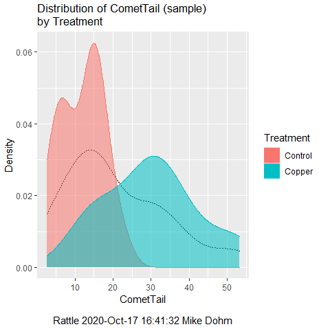
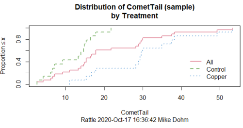
Figure 1. Rattle descriptive graphics on Comet Copper dataset. Dotted line (top image) and red line (bottom image) follow the combined observations regardless of treatment.
So, just looking at the data set, we don’t see clear evidence for a normal-like data set. The top image (Fig 1) looks stacked to the left and the cumulative plot (bottom image) is bumped in the middle, not falling on a straight line. We’ll need to investigate the assumption of normality more for this data set. We’ll begin by discussing some hypothetical points first, then return to the data set.
Goodness of fit tests of normality hypothesis
While graphics and the “eyeball test” are very helpful, you should understand that whether or not your data fits a normal distribution, that’s a testable hypothesis. The null hypothesis is that your sample distribution fits are normal distribution. In general terms, these “fit” hypotheses are viewed as “goodness of fit” tests. Often times, the test is some variation of a  problem: you have your observed (sample distribution) and you compare it to some theoretical expected value (eg, in this situation, the normal distribution). If your data fit a normal curve, then the test statistics will be close to zero.
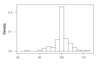
We have discussed before that the data should be from a normal distributed population. To the extent this is true, then we can trust our statistical tests are performing the way they are expected to do. We can test the assumption of normality by comparing our sample distribution against a theoretical distribution, the normal curve. I’ve shown several graphs in the past that “looked normal”. What are the alternatives for unimodal (single peak) distributions (Fig 2)?
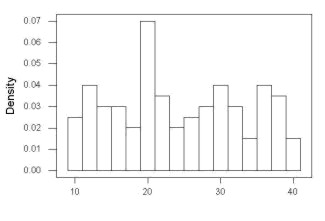
Kurtosis describes the shape of the distribution, whether it is stacked up in the middle (leptokurtosis), or more spread out and flattened (platykurtosis).
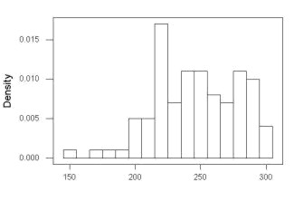
Skewness describes differences from symmetry about the middle. Left skew the tail of the distribution extends to the left, ie, smaller values.
“Leptokurtosis”
“Platykurtosis”
Negative skew, left skewed
Positive skew, right skewed
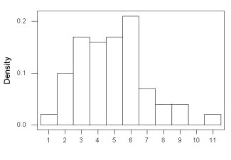
Figure 2. Graphs describing different distributions. From top to bottom: Leptokurtosis, platykurtosis, negative skew, positive skew.
The easiest procedures for goodness of fit tests of normality are based on the distribution and yield a “goodness of fit” test for normal distribution. We discussed the distribution in Chapter 6.9, and used the test in Chapter 9.1.
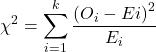
where O refers to the observed data (what we’ve got) and E refers to the expected (eg, data from a normal curve with same mean and standard deviation as our sample).
To illustrate, I simulated a data set in R.
Rcmdr: Distributions → Continuous distributions → Normal distribution → Sample from normal distribution
I created 100 values, stored them in column 1, and set the population mean = 125 and population standard deviation = 10. And therefore the population standard error of the mean was 1.0.
The resulting MIN/MAX was from 99.558 to 146.16; the sample mean was 124.59 with a sample standard deviation of 9.9164. And therefore the sample standard error of the mean was 0.9916.
Question: After completing the steps above, your data will be slightly different from mine… Why?
But getting back to the main concept, Does our data agree with a normal curve? We have discussed how to construct histograms and frequency distributions.
Let’s try six categories (why six? we discussed this when we talked about histograms).
All chi-square tests are based on categorical data, so we use the counts per category to get our data. Group the data, then count the number of OBSERVED in each group. To get the EXPECTED values, use the Z-score (normal deviate) with population mean and standard deviation as entered above.
Table 1. Tabulated values for test of normality.
| Number of observations | Weight | Normal deviate (Z) | Expected Proportion | Expected number | (Obs – Exp)2 / Exp |
| 105 | 3 | less than or equal to -2 | 0.0228 | 2.28 | 0.227368421 |
| 105 < 115 | 17 | between -1 & -2 = 0.1587 – 0.0228 | 0.1359 | 13.59 | 0.855636497 |
| 115 < 125 | 34 | between -0 & -1 = 0.5 – 0.1587 | 0.3413 | 34.13 | 0.000495166 |
| 125 < 135 | 30 | between +0 & +1 = 0.5 – 0.1587 | 0.3413 | 34.13 | 0.499762672 |
| 135 < 145 | 15 | between +1 & +2 = 0.9772 – 0.8413 | 0.1359 | 13.59 | 0.146291391 |
| > 145 | 1 | greater than or equal to +2 = 1 – 0.9772 | 0.0228 | 2.28 | 0.718596491 |
 |
Then obtain the critical value of the with df = 6 – 1 = 5 (see Appendix, Table of chi-square critical values , critical = 11.1 with df = 5).
Thus, we would not reject the null hypothesis and would proceed with the assumption that our data could have come from a normally distributed population.
This would be an OK test, but different approaches, although based on a chi-square-like goodness of fit, have been introduced and are generally preferred. We have just shown how one could use the chi-square goodness of fit approach to testing whether your data fit a normal distribution. A number of modified tests based on this procedure have been proposed; we have already introduced and used one (Wilks-Shapiro), which is easily accessed in R.
Rcmdr: Summaries → Wilks-Shapiro
Like Wilks-Shapiro, another common “goodness-of-fit” test of normality is the Anderson-Darling test. This test is now included with Rcmdr, but it’s also available in the package nortest. After the package is installed and you run the library (you should by now be able to do this!), then at the R prompt (>) type:
ad.test(dataset$variable)
replacing “dataset$variable” with the name of your data set and variable name.
In the context of goodness of fit, a perfect fit means the data are exactly distributed as a normal curve, and the test statistics would be zero. Differences away from normality increase the value of the test statistic.
How do these tests perform on data?
The histogram of our simulated normal data of 100 observations with mean = 125 and standard deviation = 10 (Fig 3).
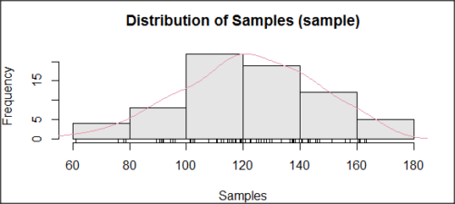
Figure 3. Histogram of simulated normal dataset, μ = 125, σ = 10.
and here’s the cumulative plot (Fig 4).
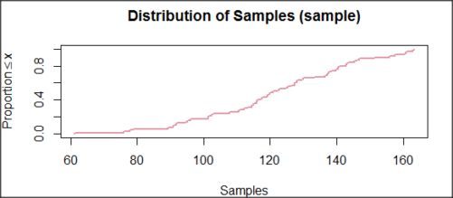
Figure 4. Cumulated frequency of simulated normal dataset, μ = 125, σ = 10.
Results from Anderson-Darling test were A = 0.2491, p-value = 0.7412, where A is the Anderson-Darling test statistic.
Results of the Shapiro-Wilks test on the same data. W = 0.9927, p-value = 0.8716, where W is the Shapiro-Wilks test statistic. We would not reject the null hypothesis in either case because p > 0.05.
Example
Histogram of a data set, highly skewed to the right. 90 observations in three groups of 30 each, with mean = 0 and standard deviation = 1 (Fig 5).
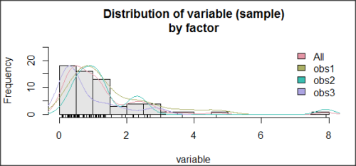
Figure 5. Histogram of simulated normal dataset, μ = 0, σ = 1.
and the cumulative frequency plot (Fig 6).
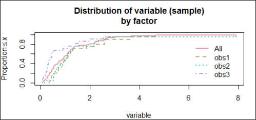
Figure 6. Cumulated frequency of simulated normal dataset, μ = 0, σ = 1.
Results from Anderson-Darling test were A = 9.0662, p-value < 2.2e-16. Results of the Shapiro-Wilks test on the same data. W = 0.6192, p-value = 6.248e-14. Therefore, we would reject the null hypothesis because p < 0.05.
The Shapiro-Wilk test in Rcmdr
Let’s go back to our data set and try tests of normality on the entire data set, ie, not by treatment groups.
Rcmdr: Statistics → Summaries → Test of normality…
normalityTest(~CometTail, test="shapiro.test", data=CometCopper)

 Shapiro-Wilk normality test

data: CometCopper$CometTail
W = 0.91662, p-value = 0.006038
End of R output
Another test, built on the basic idea of a chi-square goodness of fit is the Anderson Darling test. Some statisticians prefer this test and it is one built-in to some commercial statistical packages (eg, Minitab). To obtain the Anderson-Darling test in R, you need to install a package. After installing nortest package, run the AD test at the command prompt.
require(nortest)
ad.test(CometCopper$CometTail)

Anderson-Darling normality test

data: CometCopper$CometTail
A = 1.0833, p-value = 0.006787
End of R output.
Note
Add notes here…
Because you’ve installed Rcmdr the Anderson-Darling test is available (since version 2.6) without installing the nortest package. You can call Anderson-Darling via the menu system, Statistics → Summaries → Test of normality … or type in the script the following command
normalityTest(~CometTail, test="ad.test", data=CometCopper)
In contrast, Shapiro-Wilks test is part of the base R package, so can be called directly
shapiro.test(CometCopper$CometTail)
P-values are both much less than 0.05, so we would reject the assumption of normality for this data set.
Which test of normality?
Why show you two tests for normality, the Shapiro-Wilks and Anderson-Darling? The simple answer is that both are good as general tests of normality, both are widely used in scientific papers, so just pick one and go with it as your general test of normality.
The more complicated answer is that each is designed to be sensitive to different kinds of departure from normality. By some measures, the Shapiro-Wilks test is somewhat better (ie, more statistical power to test the null hypothesis), than other tests, but this is not something you want to get into as a beginner. So, I show both of them to you so that you are at least introduced to the concept that there are often more than one way to test a hypothesis. The bottom-line is that plots may be best!
Questions
- Work describe in this chapter involves statistical tests of the assumption of normality. It is just as important, maybe more so, to also apply graphics to take advantage of our built-in pattern recognition functions. What graphic techniques, besides histogram, should be used to view the distribution of the data?
- In R, what command would you use so that you can call the variable name,
CometTail, directly instead of having to refer to the variable asCometCopper$CometTail? - Why are Anderson-Darling, Shapiro-Wilks and other related tests referred to as “goodness of fit” tests? You may wish to review discussion in Chapter 9.1.
- The example tests presented for the Comet Copper data set were conducted on the whole set, not by treatment groups. Re-run tests of normality via
Rcmdr, but this time, select the By groups option and select Treatment.
Quiz Chapter 13.3
Test assumption of normality
Data set used in this page
| Treatment | CometTail |
|---|---|
| Control | 17.86 |
| Control | 16.52 |
| Control | 14.93 |
| Control | 14.03 |
| Control | 13.33 |
| Control | 8.81 |
| Control | 14.70 |
| Control | 9.26 |
| Control | 21.78 |
| Control | 6.18 |
| Control | 9.20 |
| Control | 5.54 |
| Control | 6.72 |
| Control | 2.63 |
| Control | 7.19 |
| Control | 5.39 |
| Control | 11.29 |
| Control | 15.44 |
| Control | 17.86 |
| Contro | l4.25 |
| Copper | 53.21 |
| Copper | 38.93 |
| Copper | 18.93 |
| Copper | 30.00 |
| Copper | 28.93 |
| Copper | 15.36 |
| Copper | 17.86 |
| Copper | 17.50 |
| Copper | 21.07 |
| Copper | 29.29 |
| Copper | 28.21 |
| Copper | 16.79 |
| Copper | 21.07 |
| Copper | 37.50 |
| Copper | 38.22 |
| Copper | 17.86 |
| Copper | 29.64 |
| Copper | 11.07 |
| Copper | 35.00 |
| Copper | 49.29 |
Chapter 13 contents
- Introduction
- ANOVA Assumptions
- Why tests of assumption are important
- Test assumption of normality
- Tests for Equal Variances
- References and suggested readings
13.1 – ANOVA Assumptions
Introduction
Like all parametric tests, assumptions are made about the data in order to justify and trust estimates and inferences drawn from ANOVA. While acknowledging the “experimental design” message suggested by the xkcd panel in Figure 1 — the presence of a large effect size between groups mitigates the technical necessities of inferential statistics — of course, not all of our projects will have such obvious results. Understanding the impact of assumptions on inference is a key concept in (bio)statistics: when the p-value is close to the Type I error rate, deviations from assumptions may reduce our confidence in the “statistical significance” of the result.

Figure 1. xkcd.com “Statistics,” https://xkcd.com/2400/.
ANOVA assumptions include:
- Data come from normal distributed population. View with a histogram or Q-Q plot. Test with Shapiro-Wilks or other appropriate goodness of fit test (see Question 1 below). Normality tests are the subject of Chapter 13.3.
- Sample size equal among groups.
- This is an example of a potentially confounding factor — If sample sizes differ, then any difference in means could be simply because of differences in sample size! This gets us into weighted versus unweighted means.
- You shouldn’t be surprised that modern implementations of ANOVA in software easily handle (adjust for) these known confounding factors. Depending on the program, you’ll see “Adjusted means,” “least squares means,” “Marginal means” etc. This just implies that the group means are compared after accounting for confounding factors.
- Importantly, as long as sample sizes among the groups are roughly equivalent, normality assumption is not a big deal (low impact on risk of Type I error).
- Independence of errors. One consequence of this assumption is that you would not view 100 repeated observations of a trait on the same subject as 100 independent data points. We’ll return to this concept more in the next two lectures. Some examples:
-
- Colorimetric assay where the signal changes over time, and you measure in order (eg, samples from group 1 first, samples from group 2 second, etc.) — this confounds group with time.
- The consequence is that you are far more likely to reject the null hypothesis, committing a Type I error.
- Let’s say you are observing running speeds of ten mongoose. However, it turns out that five of your subjects are actually from the same family, identical quintuplets! Do you really have ten subjects?
- Compare brain-body mass ratio among different species; this is a classic comparative method problem (Fig 3). Since 1985 (Felsenstein 1985), it was recognized that the hierarchical evolutionary relationships among the species must be accounted for to control for lack of independence among the taxa tested. See Phylogenetically independent contrasts, Chapter 20.12.
- Colorimetric assay where the signal changes over time, and you measure in order (eg, samples from group 1 first, samples from group 2 second, etc.) — this confounds group with time.
- Equal variances (homogeneity) among groups. See Chapter 13.4 for how to test this for multiple groups.
Impact of assumptions
R — and pretty much all statistics packages — will calculate the ANOVA table and the p-value, but it is up to you to recognize that the P-value is accurate only if the assumptions are met. Violation of the assumption of normality can lead to Type I errors occurring more often than the 5% level. What to do if the assumptions are violated?
If the violation is due to only a handful of the data, you might proceed anyway. But following a significant test for normality, we could avoid the ANOVA in favor of nonparametric alternatives (Chapter 15), or, we might try to transform the data.
Consider a histogram of brains weight measures in grams for a variety of mammals (Fig 2).
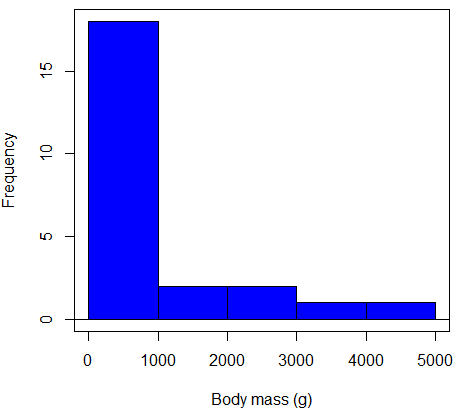
Figure 2. Histogram of body mass (g) for 24 mammals (data from Boddy et al 2012).
We will introduce a variety of statistical tests of the assumption of normality in Chapter 13.3, but looking at a histogram as part of our data exploration, we clearly see the data are right-skewed (Fig 2). Is this an example of normal distributed sample of observations? Clearly not. If we proceed with statistical tests on the raw data set, then we are more likely to commit a Type I error (ie, we will reject the null hypothesis more often than we should).
A comment on normality and biology. It is very possible that data may not be normally distributed or have equal variances on the original scale, but a simple mathematical manipulation may take care of that. In fact, in many case in biology that involve growth, many types of variables are expected to not be normal on the original scale. For example, while the relationship between body mass,  , and metabolic rate,
 , in many groups of organisms is allometric and increases positively, the relationship

is not directly proportional (linear) on the original scale. By taking the logarithm of both body mass and metabolic rate, however, the relationship is linear

In fact, taking the logarithm (base 10, base 2, or base e) is often a common solution to both non-normal data (Fig 2) and unequal variances.
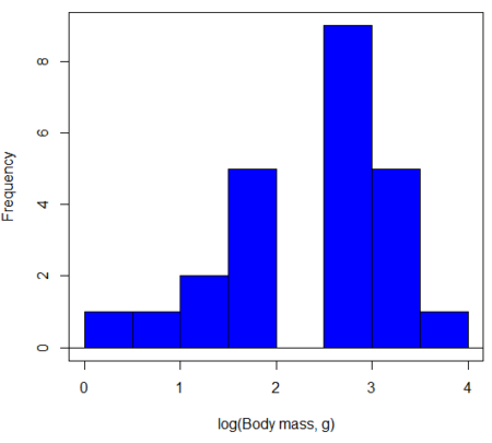
Figure 3. Histogram of log10-transformed body mass observations from Figure 2.
Other common transformations include taking the square root or the inverse of the square-root for skewed or kurtotic sample distributions, and the arcsine for frequencies (since frequencies can only be from 0 to 1 — need to “stretch the data” to make frequencies fit procedures like ANOVA). There are many issues about data transformation, but keep in mind three points. After completing the transformation, you should check the assumptions (normality, equal variances) again.
You may need to recode the data before applying a transform. For example, you cannot take the square root or logarithm of negative numbers. If you do not recode the data, then you will lose these observations in your subsequent analyses. In many cases, this problem is easily solved by adding 1 to all data points before making the transform. I prefer to make the minimum value 1 and go from there. The justification for data transformation is basically to realize that there is no necessity to use the common arithmetic or linear scale: many relationships are multiplicative or nonadditive (eg, rates in biology and medicine).
Note 1
Instead of transformations or other ad hoc manipulations of the data, modern statistical approaches favor modeling the error structure of the data within a Generalized Linear Model framework (St.-Pierre et al 2018). The advantage of the model approach is that parameter estimation occurs on the raw data. Use of transformations may, however, remain a better choice. While statistically justified, the generalized linear model approach may also tend to have higher rates of Type II error compared to simple transformations.
Statistical outlier
Another topic we should at least mention here is the concept of outliers. While most observations tend to cluster around the mean or middle of the sample distribution, occasionally one or more observations may differ substantially from the others. Such values are called outliers, and we note that there are two possible explanations for an outlier
- the value could be an error.
- it is a true value.
Note 2
“it is a true value,” and there may be an interesting biological explanation for its cause, ie, extraordinary individuals.
We encountered a clear outlier in the BMI homework. If the reason is (1), then we go back and either fix the error or delete it from the worksheet. If (2), however, then we have no objective reason to exclude the point from our analyses.
We worry if the outlier influences our conclusions — so it is a good idea to run your analyses with and without the outlier. If your conclusions remain the same, then no worries. If your conclusions change based on one observation, then this is problematic. For the most part you are then obligated to include the outlier and the more conservative interpretation of your statistical tests.
ANOVA is robust to modest deviations from assumptions
A comment about ANOVA assumptions ANOVA turns out to be robust to violations of item (1) or (2). That means unless the data are really skewed or the group sizes are very different, ANOVA will perform well (Type I error rate stays close to the specified 5% level). We worry about this however when p-value is very close to alpha!!
The third assumption is more important in ANOVA.
Like the t-test, ANOVA makes the assumption of equal variances among the groups, so it will be helpful to review why this assumption is important to both the t-test and ANOVA. In the two-sample independent t-test, the pooled sample variance,  , is taken as an estimate of the population variance,
 . If you recall,
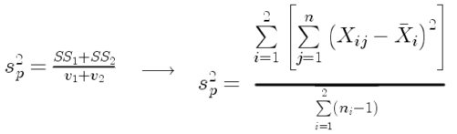
where  refers to the sum of squares for the first group and
 refers to the second group sum of squares (see our discussion on measures of dispersion) and
 refers to the degrees of freedom for the first group and
 refers to the second group degrees of freedom. We make a similar assumption in ANOVA. We assume that the variances for each sample are the same and therefore that they all estimate the population variance . To say it in another way, we are assuming that all of our samples have identical variability
Once we make this assumption, we may pool (or combine) all of the SSs and DFs for all groups as our best estimate of the population variance, . The trick to understanding ANOVA is to realize that there can be two types of variability: there is variability due to being part of a group (eg, even though ten human subjects receive the same calorie-restricted diet, not all ten will loose the same amount of weight) and there is variability among or between groups (eg, on average, all subjects who received the calorie-restricted diet lost more weight than did those subjects who were on the non-restricted diet).
Example
The encephalization index (or encephalization quotient) is defined as the ratio of size the brain compared to body size. While there is a well-recognized increase in brain size given increased body size, encephalization describes a shift of function to cortex (frontal, occipital, parietal, temporal) from noncortical parts of the brain (cerebellum, brainstem). Increased cortex is associated with increased complexity of brain function; for some researchers, the index is taken as a crude estimate of intelligence. Figure 4A shows plot of brain mass in grams versus body size (grams) for 24 mammal species (data sampled from Boddy et al 2012); Figure 4B shows the same data, but following log10-transform of both variables.
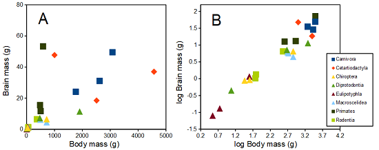
Figure 4. Plot of brain and body weights (A) and log10-log10 transform (B) for a variety of species (data from Boddy et al 2012). The ratio is called encephalization index.
Looking at the two figures the linear relationship between the two variables is obvious in Figure 4B, less so for Figure 4A. Thus, one biological justification for transformation of the raw data is exemplified with the brain-body mass dataset: the association is allometric not additive. The other reason to apply a transform is statistical; the log10-transform improves the normality of the variables. Take a look at the Q-Q plot for the raw data (Fig 5) and for the log10-transformed data (Fig 6).
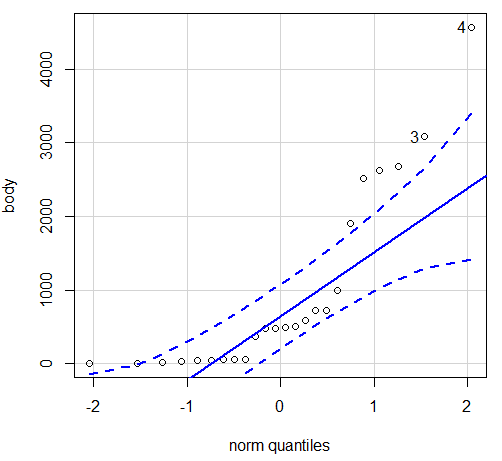
Figure 5. Q-Q plot, body mass, raw data. Compare to Figure 2.
Figure 5 is a good test of your observation skills — what are you supposed to look for in a Q-Q plot? Follow the dots — the data don’t fall on the straight line. A few even fall outside of the confidence interval (the curved dashed lines), which suggests the data were not normally distributed (see histogram, Fig 2). And for the transformed data, the Q-Q plot is shown in Figure 6.
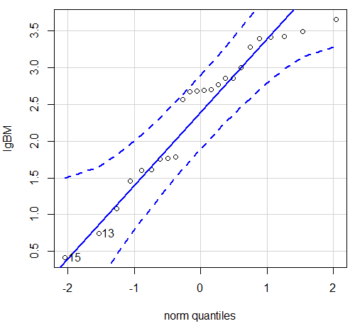
Figure 6. Q-Q plot same data, log10-transformed, compare to Figure 2.
Compared to the raw data, the transformed data now fall on the line and none are outside of the confidence interval. We would conclude that the transformed data are more normal, thus, better meeting the assumptions of our parametric tests.
Lack of independence among data
Species comparisons are common in evolutionary biology and related fields. As noted earlier, comparative data should not be treated as independent data points (discussed in 20.12 – Phylogenetically independent contrasts). For our 24 species, I plotted the estimate of the phylogeny (timetree.org), represented in Figure 7. Some species are closely related (eg the two elephant shrews, Rhynchocyon genus). Thus, because of the hierarchical, nested nature of evolution — first articulated by Charles Darwin — instead of 24 independent data points, we have eight clusters of points (see Question 4).
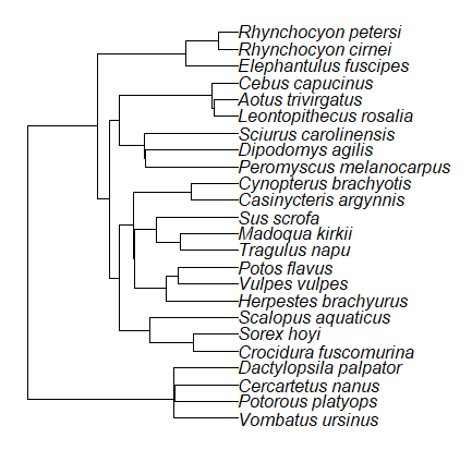
Figure 7. Phylogenetic tree of 24 species used in this report.
Note 3
The relevant quote from Charles Darwin: “… the inevitable result is that the modified descendants proceeding from one progenitor become broken up into groups subordinate to groups,” and was illustrated by the only figure in Origin of Species (both quote and illustration are in Chapter 4).
The conclusion? We don’t have 24 data points, more like 8 points. Because the species are more or less related, there are fewer than 24 independent data points. Statistically, this would mean that the errors are correlated. Various approaches to account for this lack of independence have been developed; perhaps the most common approach is to apply phylogenetically independent contrasts, a topic discussed in Chapter 20.12. (Boddy et al 2012 used this approach.)
Note 4
See 20.11 – Plot a Newick tree for how to plot phylogeny trees in R.
Questions
- Make a histogram for the brain mass data set.
- Shapiro-Wilks is one test of normality.
- Can you recall the name of the other normality tests we named?
- Run tests of normality on both body mass and brain mass data. Interpret the results, frame your response with keywords: “central tendency,” “outliers,” “shape,” and “symmetry.”
- Calculate moment statistics for the body mass and brain mass data set, both raw and log10-transformed data. Interpret your results, taking care to frame your answer with the following keywords: “shape,” “symmetry,” and “peakedness” (aka “tailedness”).
- We introduced the lack of independence for comparative data attributed to the evolutionary process. Statistically, the impact is on degrees of freedom; for example, if we ignore the lack of independence in the data set, df = 22 for the slope coefficient in a linear regression. However, given the degrees of freedom would be closer to six! What are the effects on Type I error rate of lack of independence?
Quiz Chapter 13.1
ANOVA assumptions
Data set and R code used in this page
species, order, body, brain
'Herpestes ichneumon', Carnivora, 1764, 24.1
'Potos flavus', Carnivora, 2620, 31.05
'Vulpes vulpes', Carnivora, 3080, 49.5
'Madoqua kirkii', Cetartiodactyla, 4570, 37
'Sus scrofa', Cetartiodactyla, 1000, 47.7
'Tragulus napu', Cetartiodactyla, 2510, 18.5
'Casinycteris argynnis', Chiroptera, 40.5, 0.92
'Cynopterus brachyotis', Chiroptera, 29, 0.88
'Potorous platyops', Chiroptera, 718, 6.5
'Cercartetus nanus', Diprotodontia, 12, 0.44548
'Dactylopsila palpator', Diprotodontia, 474, 7.15876
'Vombatus ursinus', Diprotodontia, 1902, 11.396
'Crocidura fuscomurina', Eulipotyphla, 5.6, 0.13
'Scalopus aquaticus', Eulipotyphla, 39.6, 1.48
'Sorex hoyi', Eulipotyphla, 2.6, 0.107
'Elephantulus fuscipes', Macroscelidea, 57, 1.33
'Rhynchocyon cirnei', Macroscelidea, 490, 6.1
'Rhynchocyon petersi', Macroscelidea, 717.3, 4.46
'Aotus trivirgatus', Primates, 480, 15.5
'Cebus capucinus', Primates, 590, 53.28
'Leontopithecus rosalia', Primates, 502.5, 11.7
'Dipodomys agilis', Rodentia, 61.4, 1.34
'Peromyscus melanocarpus', Rodentia, 58.8, 1.03
'Sciurus carolinensis', Rodentia, 367, 6.49
The Newick code for the tree in Figure 6.
((Vombatus_ursinus:48.94499077,((Potorous_platyops:47.59556667,Cercartetus_nanus:47.59556667)'14':0.66887333,Dactylopsila_palpator:48.26444000)'13':0.68055077)'11':109.65259681,(((((Crocidura_fuscomurina:33.74066667,Sorex_hoyi:33.74066667)'10':33.03022424,Scalopus_aquaticus:66.77089091)'19':22.55292749,(((Herpestes_brachyurus:54.32144118,(Vulpes_vulpes:45.52834967,Potos_flavus:45.52834967)'9':8.79309151)'22':23.43351523,((Tragulus_napu:43.96862857,Madoqua_kirkii:43.96862857)'8':17.99735995,Sus_scrofa:61.96598852)'6':15.78896789)'30':0.77378567,(Casinycteris_argynnis:35.20000000,Cynopterus_brachyotis:35.20000000)'29':43.32874208)'27':10.79507632)'35':7.13857077,(((Peromyscus_melanocarpus:69.89837667,Dipodomys_agilis:69.89837667)'43':0.64655123,Sciurus_carolinensis:70.54492789)'42':19.27825952,((Leontopithecus_rosalia:18.38385647,Aotus_trivirgatus:18.38385647)'40':1.29720005,Cebus_capucinus:19.68105652)'48':70.14213090)'51':6.63920175)'47':8.99739162,(Elephantulus_fuscipes:39.23366667,(Rhynchocyon_cirnei:15.34500000,Rhynchocyon_petersi:15.34500000)'39':23.88866667)'56':66.22611412)'55':53.13780679);
Chapter 13 contents
8.1 – The null and alternative hypotheses
Introduction
Classical statistical parametric tests — t-test (one sample t-test, independent sample-t-test), analysis of variance (ANOVA), correlation, and linear regression— and nonparametric tests like (chi-square: goodness of fit and contingency table), share several features that we need to understand. It’s natural to see all the details as if they are specific to each test, but there’s a theme that binds all of the classical statistical inference in order to make claim of “statistical significance.”
- a calculated test statistic
- degrees of freedom associated with the calculation of the test statistic
- a probability value or p-value which is associated with the test statistic, assuming a null hypothesis is “true” in the population from which we sample.
- Recall from our previous discussion (Chapter 8.2) that this is not strictly the interpretation of p-value, but a short-hand for how likely the data fit the null hypothesis. P-value alone can’t tell us about “truth.”
- in the event we reject the null hypothesis, we provisionally accept the alternative hypothesis.
Statistical Inference in the NHST Framework
By inference we mean to imply some formal process by which a conclusion is reached from data analysis of outcomes of an experiment. The process at its best leads to conclusions based on evidence. In statistics, evidence comes about from the careful and reasoned application of statistical procedures and the evaluation of probability (Abelson 1995).
Formally, statistics is rich in inference process (Bzdok et al, 2018). We begin by defining the classical frequentist, aka Neyman-Pearson approach, to inference, which involves the pairing of two kinds of statistical hypotheses: the null hypothesis (HO) and the alternative hypothesis (HA). The null hypothesis assumes that any observed difference between the groups are the results of random chance (introduced in Ch 2.3 – A brief history of (bio)statistics ), where “random chance” implies that outcomes occur without order or pattern (Eagle 2021). Whether we reject or accept the null hypothesis — a short-hand for the more appropriate “provisionally reject” in light of the humility that our results may reflect a rare sampling event — based on the outcome of our statistical inference, the inference is evaluated against a decision criterion (cf discussion in Christiansen 2005), a fixed statistical significance level (Lehmann 1992). Significance level refers to the setting of a p-value threshold before testing is done. The threshold is often set to Type I error of 5% (Cowles & Davis 1982), but researchers should always consider whether this threshold is appropriate for their work (Benjamin et al 2017).
This inference process is referred to as Null Hypothesis Significance Testing, NHST. Additionally, a probability value will be obtained for the test outcome or test statistic value. In the Fisherian likelihood tradition, the magnitude of this statistic value can be associated with a probability value, the p-value, of how likely the result is given the null hypothesis is “true.” (Again, keep in mind that this is not strictly the interpretation of p-value, it’s a short-hand for how likely the data fit the null hypothesis. P-value alone can’t tell us about “truth”, per our discussion, Chapter 8.2.)
Note 1
About reporting p-values, -logP. A Google search will likely reveal “logP,” which is a measure in chemistry. In contrast, “-logP” pertains to how to report p-values in statistics. P-values are traditionally reported as a decimal, like 0.000134, in the closed (set) interval (0,1) — p-values can never be exactly zero or one. The smaller the value, the less the chance our data agree with the null prediction. Small numbers like this can be confusing, particularly if many p-values are reported, like in many genomics works, eg, GWAS studies. In the past, small p-values would be reported as “less than,” eg, < 0.001. This was done in part because of the misleading impression of precision that many significant figures can represent (see discussion in Lang and Altman 2014).
-logP is an alternative, particularly for GWAS studies where the significance level may be much smaller than 5%. Thus, instead of reporting vanishingly small p-values, studies may report the negative log10 p-value, or -logP. Instead of small numbers, large numbers are reported, the larger, the more against the null hypothesis. Thus, our p-value becomes 3.87 -logP.
R code
-1*log(0.000134,10)
[1] 3.872895
Why log10 and not some other base transform? Just that log10 is convenience — powers of 10.
The antilog of 3.87 returns our p-value
> 10^(-1*3.872895)
[1] 0.0001340001
For convenience, a partial p-value -logP transform table
| P-value | -logP |
| 0.1 | 1 |
| 0.01 | 2 |
| 0.001 | 3 |
| 0.0001 | 4 |
On your own, complete the table up to -logP 5 – 10. See Question 7 below.
NHST Workflow
We presented in the introduction to Chapter 8 without discussion a simple flow chart to illustrate the process of decision (Fig 1, Chapter 8). Here, we repeat the flow chart diagram and follow with descriptions of the elements.
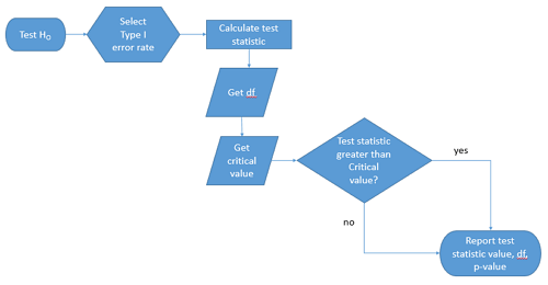
Figure 1. Flow chart of inductive statistical reasoning.
What’s missing from the flow chart is the very necessary caveat that interpretation of the null hypothesis is associated with two kinds of error, Type I error and Type II error. These points and others are discussed in the following sections.
We start with the hypothesis statements. For illustration we discuss hypotheses in terms of comparisons involving just two groups, also called two sample tests. One sample tests in contrast refer to scenarios where you compare a sample statistic to a population value. Extending these concepts to more than two samples is straightforward, but we leave that discussion to Chapters 12 – 18.
Null hypothesis
By far the most common application of the null hypothesis testing paradigm involves the comparisons of different treatment groups on some outcome variable. These kinds of null hypotheses are the subject of Chapters 8 through 12.
The Null hypothesis (HO) is a statement about the comparisons, eg, between a sample statistic and the population, or between two treatment groups. The former is referred to as a one tailed test whereas the latter is called a two-tailed test. The null hypothesis is typically “no statistical difference” between the comparisons.
For example, a one sample, two tailed null hypothesis.

and we read it as “there is no statistical difference between our sample mean and the population mean.” For the more likely case in which no population mean is available, we provide another example, a two sample, two tailed null hypothesis.

Here, we read the statement as “there is no difference between our two sample means.” Equivalently, we interpret the statement as both sample means estimate the same population mean.

Under the Neyman-Pearson approach to inference we have two hypotheses: the null hypothesis and the alternative hypothesis. The hull hypothesis was defined above.
Note 2
Tails of a test are discussed further in chapter 8.4.
Alternative hypothesis
Alternative hypothesis (HA): If we conclude that the null hypothesis is false, or rather and more precisely, we find that we provisionally fail to reject the null hypothesis, then we provisionally accept the alternative hypothesis. The view then is that something other than random chance has influenced the sample observations. Note that the pairing of null and alternative hypotheses covers all possible outcomes. We do not, however, say that we have evidence for the alternative hypothesis under this statistical regimen (Abelson 1995). We tested the null hypothesis, not the alternative hypothesis. Thus, it is incorrect to write that, having found a statistical difference between two drug treatments, say aspirin and acetaminophen for relief of migraine symptoms, it is not correct to conclude that we have proven the case that acetaminophen improves improves symptoms of migraine sufferers.
For the one sample, two tailed null hypothesis, the alternative hypothesis is

and we read it as “there is a statistical difference between our sample mean and the population mean.” For the two sample, two tailed null hypothesis, the alternative hypothesis would be

and we read it as “there is a statistical difference between our two sample means.”
Alternative hypothesis often may be the research hypothesis.
It may be helpful to distinguish between technical hypotheses, scientific hypothesis, or the equality of different kinds of treatments. Tests of technical hypotheses include the testing of statistical assumptions like normality assumption (see Chapter 13.3) and homogeneity of variances (Chapter 13.4). The results of inferences about technical hypotheses are used by the statistician to justify selection of parametric statistical tests (Chapter 13). The testing of some scientific hypothesis like whether or not there is a positive link between lifespan and insulin-like growth factor levels in humans (Fontana et al 2008), like the link between lifespan and IGFs in other organisms (Holtzenberger et al 2003), can be further advanced by considering multiple hypotheses and a test of nested hypotheses and evaluated either in Bayesian or likelihood approaches (Chapter 16 and Chapter 17). The advantage of the Bayesian approach is that it returns evidence for or against this hypothesis: if the posterior probability is greater than the prior probability, we can we say that we have evidence for the hypothesis. This is very appealing — the challenge is that the prior probability is inherently subjective (Chapter 6.4), limited by the amount and quality of existing information pertaining to the hypothesis (Prelec 2004).
Note 3
In Bayesian statistics, hypotheses and their parameters are treated as random variables and we can assign them probabilities. The prior probability is your initial belief about the likelihood of an event before adding new data. The posterior probability is the updated probability after new data has been added. Thus, the posterior combines your prior belief with the new information (the likelihood).
In the frequentis approach, the null hypothesis is no difference (no effect); in the Bayesian context, we’d treat this as a point estimate of zero and have to assign it a probability. In the absence of empirical evidence, one option is to set the probability as 50%, equal prior odds. Use of the spike and slab prior is likely a better approach. There’s a lot of work on these points; I refer interested readers to Campbell and Gustafson (2024) for additional readings and discussion.
How to interpret the results of a statistical test.
Any number of statistical tests may be used to calculate the value of the test statistic. For example, a one sample t-test may be used to evaluate the difference between the sample mean and the population mean (Chapter 8.5) or the independent sample t-test may be used to evaluate the difference between means of the control group and the treatment group (Chapter 10). The test statistic is the particular value of the outcome of our evaluation of the hypothesis and it is associated with the p-value. In other words, given the assumption of a particular probability distribution, in this case the t-distribution, we can associate a probability, the p-value, that we observed the particular value of the test statistic and the null hypothesis is true in the reference population.
By convention, we determine statistical significance (Cox 1982; Whitley & Ball 2002) by assigning ahead of time a decision probability called the Type I error rate, often given the symbol α (alpha). The practice is to look up the critical value that corresponds to the outcome of the test with degrees of freedom like your experiment and at the Type I error rate that you selected. The Degrees of Freedom (DF, df, or sometimes noted by the symbol v), are the number of independent pieces of information available to you. Knowing the degrees of freedom is a crucial piece of information for making the correct tests. Each statistical test has a specific formula for obtaining the independent information available for the statistical test. We first were introduced to DF when we calculated the sample variance with the Bessel correction, n – 1, instead of dividing through by n. With the df in hand, the value of the test statistic is compared to the critical value for our null hypothesis. If the test statistic is smaller than the critical value, we fail to reject the null hypothesis. If, however, the test statistic is greater than the critical value, then we provisionally reject the null hypothesis. This critical value comes from a probability distribution appropriate for the kind of sampling and properties of the measurement we are using. In other words, the rejection criterion for the null hypothesis is set to a critical value, which corresponds to a known probability, the Type I error rate.
Before proceeding with yet another interpretation, and hopefully less technical discussion about test statistics and critical values, we need to discuss the two types of statistical errors. The Type I error rate is the statistical error assigned to the probability that we may reject a null hypothesis as a result of our evaluation of our data when in fact in the reference population, the null hypothesis is, in fact, true. In Biology we generally use Type I error α = 0.05 level of significance. We say that the probability of obtaining the observed value AND HO is true is 1 in 20 (5%) if α = 0.05. Put another way, we are willing to reject the Null Hypothesis when there is only a 5% chance that the observations could occur and the Null hypothesis is still true. Our test statistic is associated with the p-value; the critical value is associated with the Type I error rate. If and only if the test statistic value equals the critical value will the p-value equal the Type I error rate.
The second error type associated with hypothesis testing is, β, the Type II statistical error rate. This is the case where we accept or fail to reject a null hypothesis based on our data, but in the reference population, the situation is that indeed, the null hypothesis is actually false. We must also keep in mind that, as we evaluate the p-value relative to the magnitude of the Type I error rate, and if we reject the null hypothesis, we still do not say that we have evidence for the alternative hypothesis.
Thus, we end with a concept that may take you a while to come to terms with — there are four, not two possible outcomes of an experiment.
Outcomes of an experiment
What are the possible outcomes of a comparative experiment? We have two treatments, one in which subjects are given a treatment and the other, subjects receive a placebo. Subjects are followed and an outcome is measured. We calculate the descriptive statistics aka summary statistics, means, standard deviations, and perhaps other statistics, and then ask whether there is a difference between the statistics for the groups. So, two possible outcomes of the experiment, correct? If the treatment has no effect, then we would expect the two groups to have roughly the same values for means, etc., in other words, any difference between the groups is due to chance fluctuations in the measurements and not because of any systematic effect due to the treatment received. Conversely, then if there is a difference due to the treatment, we expect to see a large enough difference in the statistics so that we would notice the systematic effect due to the treatment.
Actually, there are four, not two, possible outcomes of an experiment, just as there were four and not two conclusions about the results of a clinical assay. The four possible outcomes of a test of a statistical null hypothesis are illustrated in Table 1.
Table 1. When conducting hypothesis testing, four outcomes are possible.
| HO in the population | |||
| True | False | ||
| Result of statistical test | Reject HO | Type I error with probability equal to
α (alpha) |
Correct decision, with probability equal to
1 – β (1 – beta) |
| Fail to reject the HO | Correct decision with probability equal to
1 – α (1 – alpha) |
Type II error with probability equal to
β (beta) |
|
In the actual population, a thing happens or it doesn’t. The null hypothesis is either true or it is not. But we don’t have access to the reference population, we don’t have a census. In other words, there is truth, but we don’t have access to the truth. We can weight, assigned as a probability or p-value, our decisions by how likely our results are given the assumption that the truth is indeed “no difference.”
If you recall, we’ve seen a table like Table 1 before in our discussion of conditional probability and risk analysis (Chapter 7.3). We made the point that statistical inference and the interpretation of clinical tests are similar (Browner and Newman 1987). From the perspective of ordering a diagnostic test, the proper null hypothesis would be the patient does not have the disease. For your review, here’s that table (Table 2).
Table 2. Interpretations of results of a diagnostic or clinical test.
| Does the person have the disease? | |||
| Yes | No | ||
| Result of the diagnostic test |
Positive | sensitivity of the test (a) | False positive (b) |
| Negative | False negative (c) | specificity of the test (d) | |
Thus, a positive diagnostic test result is interpreted as rejecting the null hypothesis. If the person actually does not have the disease, then the positive diagnostic test is a false positive.
Questions
- Match the corresponding entries in the two tables. For example, which outcome from the inference/hypothesis table matches specificity of the test?
- Find three sources on the web for definitions of the p-value. Write out these definitions in your notes and compare them.
- In your own words distinguish between the test statistic and the critical value.
- All of our discussions have been about testing the null hypothesis, about accepting or rejecting, provisionally, the null hypothesis.
- What are the p-values for -logP of 5, 6, 7, 8, 9, and 10? Complete the p-value -logP transform table.
- Instead of log10 transform, create a similar table but for negative natural log transform. Which is more convenient? Hint:
log(x, base=exp(1))
Quiz Chapter 8.1
The null and alternate hypothesis