20.13 – How to get the distances from a distance tree
Introduction
Extract the patristic distance, the sum of the branch lengths that link two nodes in a tree, for each pair of species.
This distance — see our Chapter 16.6 – Similarity and Distance— is the proportion (p) of amino acid (or nucleotide for DNA or RNA) sites at which the two sequences to be compared are different. It is obtained by dividing the number of amino acid differences by the total number of sites compared. It does not make any correction for multiple substitutions at the same site or differences in evolutionary rates among sites. On a gene tree (Fig. 1), distances are the lengths of the branches connecting the taxa. We want to know how different are two species for the given protein? That’s the distance between them in proportion of amino acid sites that are different by total number compared.
Example
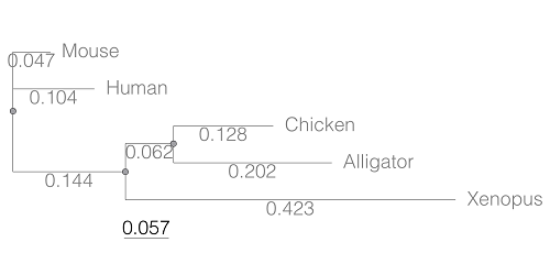
Figure 1. A gene tree of the product (protein HBA1) with five species.
Here’s the Newick format for the tree (HBA1.nwk)
(Mouse:0.0474516,Human:0.104063,((Chicken:0.127652,Alligator:0.202421):0.0616593,Xenopus:0.422801):0.143939);
R code to extract distances and output sorted, pairwise comparisons to a text file
library(ape)

# Create a function
getDis <- function(tree, tips) {
     myTree <- cophenetic(tree)
     myTree <- myTree[,tips]
     xy <- t(combn(colnames(myTree), 2))
     xy <- xy[order(xy[,1], xy[,2]),]
     myOut <- data.frame(xy, myTree[xy])
     colnames(myOut) <- c("Spp1", "Spp2", "Distance")
   return(myOut)
}

# Read a tree file, Newick format
tree5 <-read.tree(text="(Mouse:0.0474516,Human:0.104063,((Chicken:0.127652,Alligator:0.202421):0.0616593,Xenopus:0.422801):0.143939);")

# get taxa names from the tree file
all.tips <- tree5$tip.label; all.tips

# Run the function
myDis <- getDis(tree5, all.tips)

# Check the output
head(myDis)

# Create the results file
write.csv(myDis, file = "my_out.txt")
Example output from head(myDist)
       Spp1    Spp2  Distance
1 Alligator Xenopus 0.6868813
2 Chicken Alligator 0.3300730
3 Chicken   Xenopus 0.6121123
4 Human   Alligator 0.5120823
5 Human     Chicken 0.4373133
6 Human     Xenopus 0.6708030
The function sorts first by Spp1, then by Spp2.
Molecular clock plot
Collect divergence times from timetree.org
| Spp1 | Spp2 | Time (median MYA) |
| Alligator | Xenopus | 352 |
| Chicken | Alligator | 245 |
| Chicken | Xenopus | 352 |
| Human | Alligator | 319 |
| Human | Chicken | 319 |
| Human | Xenopus | 352 |
A scatterplot of distance HBA protein sequence by log10-transformed millions of years ago divergence time shown in Figure 2. Note, although tempting, calculating the slope from a linear regression to estimate the rate of evolution would not be appropriate without accounting for the lack of independence of the data (see Phylogenetically independent contrasts). Better methods exist, including calculating rate of change after fitting a model that assumes a strict clock vs relaxed clock.
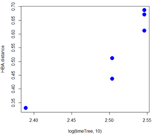
Figure 2. Scatterplot HBA distance by logMYA divergence time
Questions
[pending]
Suggested readings
Bevan, R. B., Lang, B. F., & Bryant, D. (2005). Calculating the evolutionary rates of different genes: a fast, accurate estimator with applications to maximum likelihood phylogenetic analysis. Systematic biology, 54(6), 900-915.
Chapter 20 contents
- Additional topics
- Area under the curve
- Peak detection
- Baseline correction
- Surveys
- Time series
- Dimensional analysis
- Estimating population size
- Diversity indexes
- Survival analysis
- Growth equations and dose response calculations
- Plot a Newick tree
- Phylogenetically independent contrasts
- How to get the distances from a distance tree
- Binary classification
- Meta-analysis
/MD
20.12 – Phylogenetically independent contrasts
Introduction
Assumption of independence among the subjects in a study, key assumption. Cross species comparisons as tests of correlated evolution of traits has a long history in biology research (Cornwallis and Griffin 2024). Methods have transitioned from observations to rigorous, phylogenetic tree-based statistical approaches (phylogenetic comparative methods), and continue to provide important analytical tools, eg., host adaptation and cross-species transmission of Covid-19 virus (Attwood et al 2022).
Comparisons among species for the association between body size and metabolic rate, for example Kleiber’s Law, are classic cases (Fig 1, after Table 2 in Kleiber 1947). We’ll use Kleiber’s data basal metabolic rate (BMR) and body mass for a collection of species to explore two phylogenetic comparative methods, PIC and PGLS.
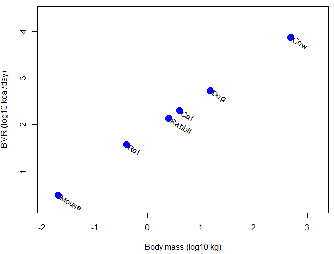
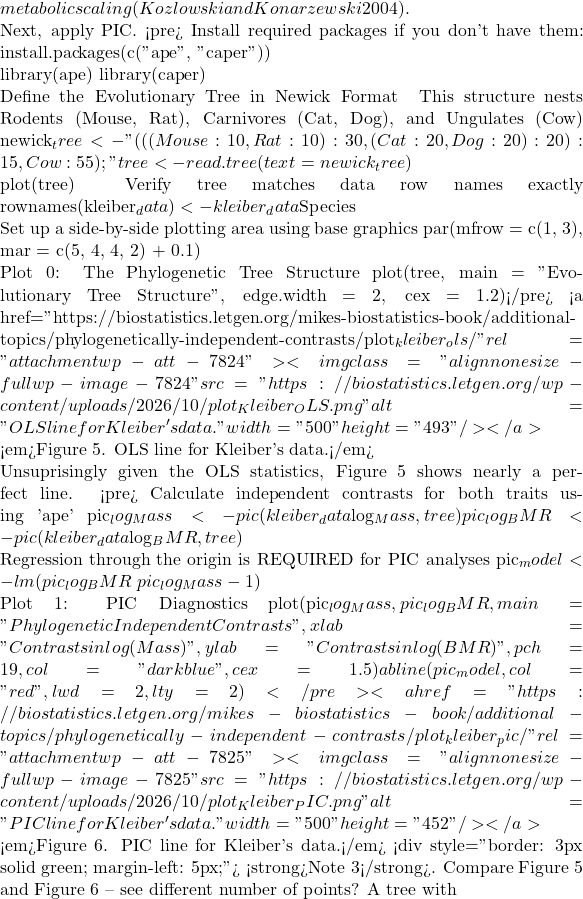
Figure 1. Scatter plot of BMR on Body Mass, log-transformed.
Typical approaches statistically, use of ANOVA or linear regression approaches. A basic assumption of ANOVA is that sampling units are independent 13.1 – ANOVA assumptions.
Prior to the 1980s, it was rarely appreciated in comparative analysis that species are not independent sample units (Harvey and Pagel 1991); evolution produced nested hierarchical relationships among the species. We recognize this with phylogenies (Felsenstein 1985, Harvey and Pagel 1991, Martins 1996, Garland et al 2005). Mice and rats share more recent common ancestor, and cattle and pigs share more recent common ancestor, than do mice and cattle, for example. Felsenstein (1985, 1988), largely credited for making the argument that Type I error likely if phylogeny ignored, and, importantly, provided an algorithm, Phylogenetic Independent Contrasts, PIC, which provided a simple way to correct for phylogenetic nonindependence. Felsentein’s landmark 1985 paper has been cited more than ten thousand times (Feb 2024).
Logic of PIC
Treating comparative data, eg, species, as a collection of independent samples implies that the evolutionary history was a spontaneous burst, or star-like phylogeny — an unresolved phylogenetic tree with branches radiating from a single ancestral node (Fig 2).
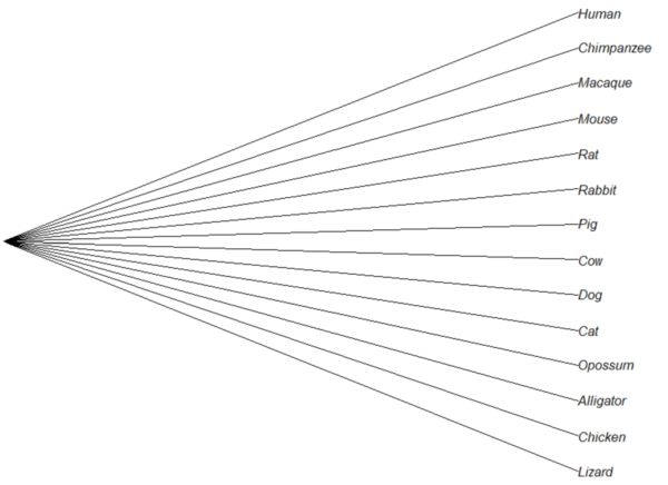
Figure 2. Star tree phylogeny (same image shown Figure 5, 20.11 – Plot a Newick tree).
But what nature provides is nonindependence (Fig 3, for more about star phylogeny in PIC see discussion in Garland et al 2005), Darwin’s “groups under groups,” or a nested hiearchy. Species are not independent units and phylogenetic history should be accounted for during statistical analysis.
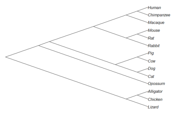
Figure 3. A cladogram for same species, showing the hierarchical, nested relationships among taxa, what nature actually provides (same image shown Figure 2, 20.11 – Plot a Newick tree).
Let’s revisit Figure 1. What do the points look like if we line up the known phylogeny for Kleiber’s six species against the plotted data? That gives us Figure 4.
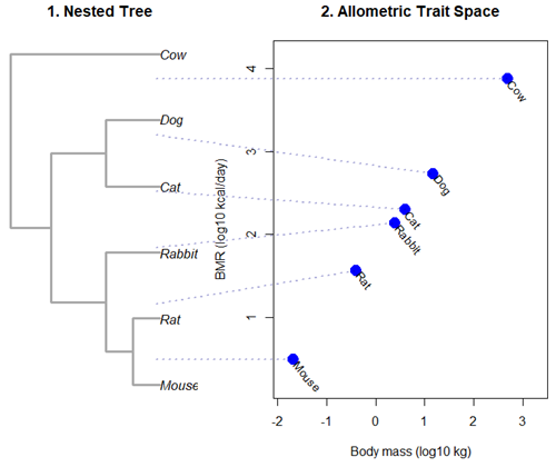
Figure 4. Kleiber’s Law and the confounding effect of shared ancestry.
Dashed connecting lines in Figure 4 trace each species from its tree position to its phenotypic value, demonstrating how phylogenetic clustering violates the independent data assumptions of standard OLS regression.
Begin R code for Figure 4, with remarks — code generated with Gemini AI assistance.
# 1. Reset the data frame
kleiber_data <- data.frame(
Species = c("Mouse", "Rat", "Rabbit", "Cat", "Dog", "Cow"),
Mass = c(0.021, 0.282, 2.45, 3.1, 13.4, 439.0),
BMR = c(3.38, 32.4, 134.0, 151.0, 506.0, 6135.0),
stringsAsFactors = FALSE
)
kleiber_data$log_Mass <- log10(kleiber_data$Mass)
kleiber_data$log_BMR <- log10(kleiber_data$BMR)

# 2. Build the exact matching standalone 6-species tree
library(ape)
newick_tree_6 <- "((((Mouse:10,Rat:10):10,Rabbit:20):20,(Cat:20,Dog:20):20):15,Cow:55);"
my_tree <- read.tree(text = newick_tree_6)

# 3. Setup a side-by-side 2-panel layout
layout(matrix(c(1, 2), nrow = 1), widths = c(1, 1.3))
par(mar = c(5, 4, 4, 1))

# PANEL 1: Plot the tree hierarchy
plot(my_tree, main = "1. Nested Tree",
edge.width = 3, edge.color = "darkgrey", cex = 1.1)

# FIXED COORDINATE MAP: 'ape' plots leaves bottom-to-top exactly matching the tree order
# We map the tree tip labels to simple integers 1 through 6
tree_heights <- 1:6
names(tree_heights) <- my_tree$tip.label

# PANEL 2: Plot the scatterplot
plot(kleiber_data$log_BMR ~ kleiber_data$log_Mass,
pch = 19, cex = 2, col = "blue",
xlab = "Body mass (log10 kg)", ylab = "BMR (log10 kcal/day)",
xlim = c(min(kleiber_data$log_Mass) - 0.2, max(kleiber_data$log_Mass) + 0.6),
ylim = c(min(kleiber_data$log_BMR) - 0.3, max(kleiber_data$log_BMR) + 0.3),
main = "2. Allometric Trait Space")

# Re-apply your custom 310-degree slanted text labels
text(kleiber_data$log_Mass + 0.05, kleiber_data$log_BMR - 0.03,
labels = kleiber_data$Species, srt = 310, adj = 0, cex = 0.9, col = "black")

# 4. CROSS-PANEL LINE CORRECTION: Draw lines across the margins safely
par(xpd = NA) # Tells R to ignore the borders of the active scatterplot window

# Calculate the left-hand margin boundaries based on the current plot limits
left_x_boundary <- min(kleiber_data$log_Mass) - 2.8

for(i in 1:nrow(kleiber_data)) {
sp <- kleiber_data$Species[i]

# A. Use a standardized geometric multiplier to align with Panel 1's vertical axis
# This formula maps the tree heights (1-6) into the scatterplot's Y coordinate scale
y_scale_factor <- (tree_heights[sp] - 1) / 5
y_span_range <- max(kleiber_data$log_BMR) - min(kleiber_data$log_BMR)
target_tree_y <- min(kleiber_data$log_BMR) + (y_scale_factor * y_span_range)

# B. Pull the actual coordinates of your blue dot
right_x <- kleiber_data$log_Mass[i]
right_y <- kleiber_data$log_BMR[i]

# C. Draw a clean, connecting line directly out to the dot
segments(x0 = left_x_boundary,
y0 = target_tree_y,
x1 = right_x,
y1 = right_y,
col = adjustcolor("darkblue", alpha.f = 0.3),
lty = 3, lwd = 2)
}

# Reset layout parameters back to normal
layout(1)
End R code.
Note 1. About the code for Figure 3. Ideally, we would use the function phylomorphospace (phytools package) to superimpose the nested tree and the plot of Kleiber’s data. For example, our code would look like
R code
library(phytools)
phylomorphospace(my_tree, trait_matrix,
label = "off", # Suppresses default horizontal text labels safely
xlab = "Body mass (log10 kg)",
ylab = "BMR (log10 kcal/day)",
xlim = c(min(kleiber_data$log_Mass) - 0.2, max(kleiber_data$log_Mass) + 0.6),
ylim = c(min(kleiber_data$log_BMR) - 0.3, max(kleiber_dat$log_BMR) + 0.3),
control = list(col.edge = "darkgrey", lwd = 3))
End R code.
However, the relationship is so perfect here that the tree lies flat on the regression line so we can’t see the tree for the line, hence our use of segments().
Phylogenetic Generalized Least Squares (PGLS).
However, like most innovations, PIC should not be blindly applied in all comparative analysis (eg, unreplicated evolutionary events, Uyeda et al 2018). Fundamentally, PIC is mathematically limited: it primarily handled simple two-variable correlations and required fully resolved, bifurcating evolutionary trees with known branch lengths. At about the same time, Grafen (1989) proposed that phylogenetic non-independence could be treated as a form of spatial autocorrelation — that is, near things are more related than distant things. Instead of computing data contrasts at individual tree nodes, Grafen introduced the phylogenetic regression, which used Generalized Least Squares (GLS) to alter how the regression algorithm treats the residual errors of species data. Improvements to phylogenetic regression are now collectively refered to as the Phylogenetic Generalized Least Squares (PGLS) (Rohlf 2001, Housworth et al 2004, Mazel et al 2016, Adams et al 2019).
Logic of PGLS.
In standard Ordinary Least Squares (OLS) regression, the residual error terms (ε) are assumed to be independent and identically distributed. In matrices, this error structure is represented by an identity matrix (I), where the off-diagonals are zero, implying that knowing about the trait value of a mouse reveals no information about the value for a rat or other rodent species.
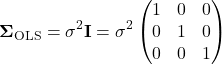
Note 2. The identity matrix  3 \times 3
 n = 3
 \sigma^{2} \times 1 = \sigma^{2}
 \sigma^{2} \times 0 = 0
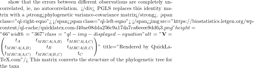
A B
 C
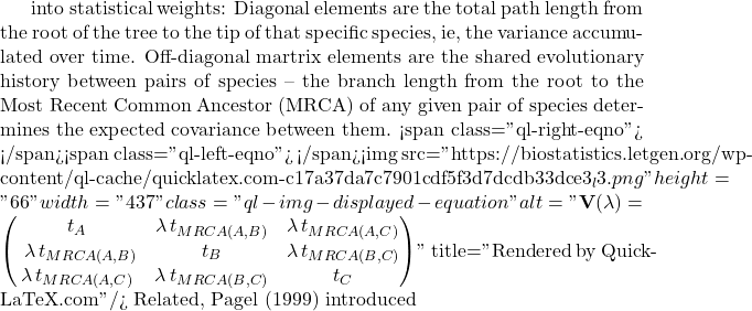
lambda Pagel’s \ \lambda
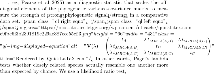
LRT \lambda

LR \chi ^{2}

\ln L_{\lambda = 0} \ln L_{\hat{\lambda}}
 \lambda
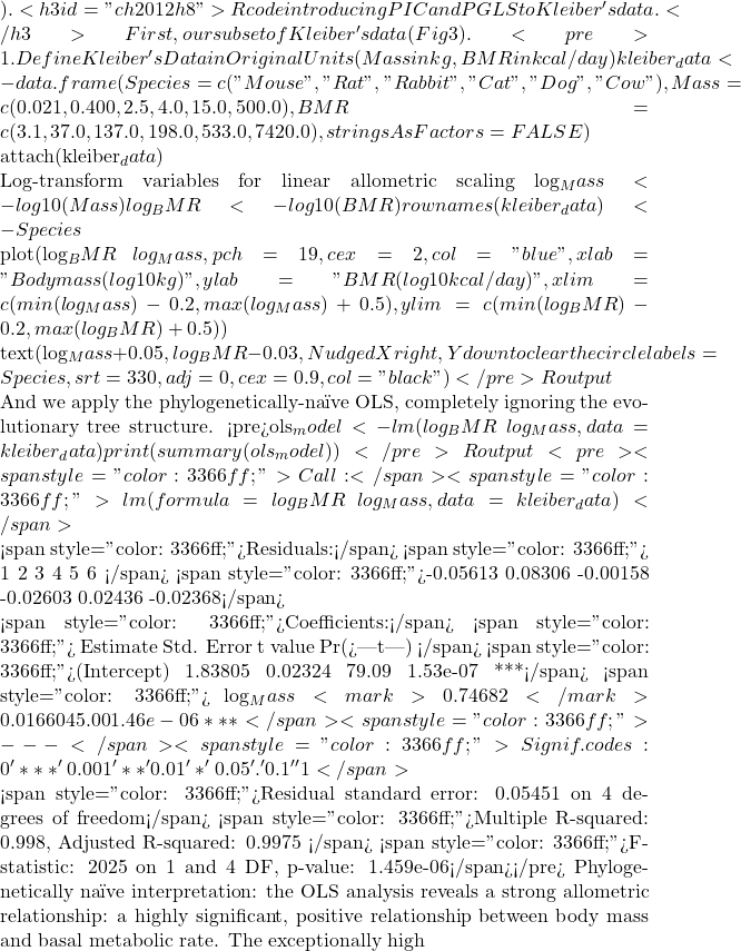 R^{2}
 BMR = aM^{b}
 \frac{3}{4}
 n
 n – 1
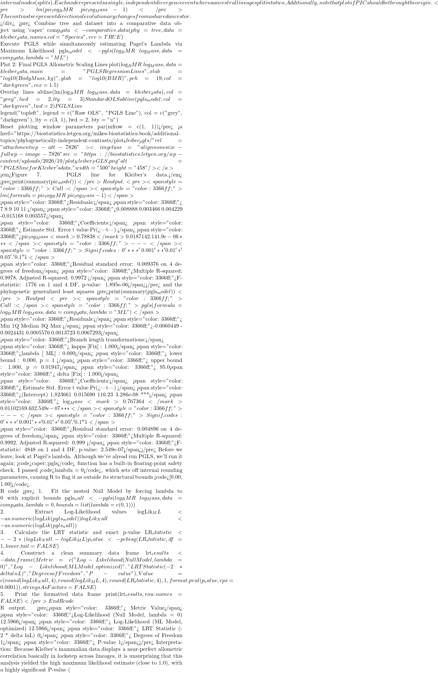 P < 0.05
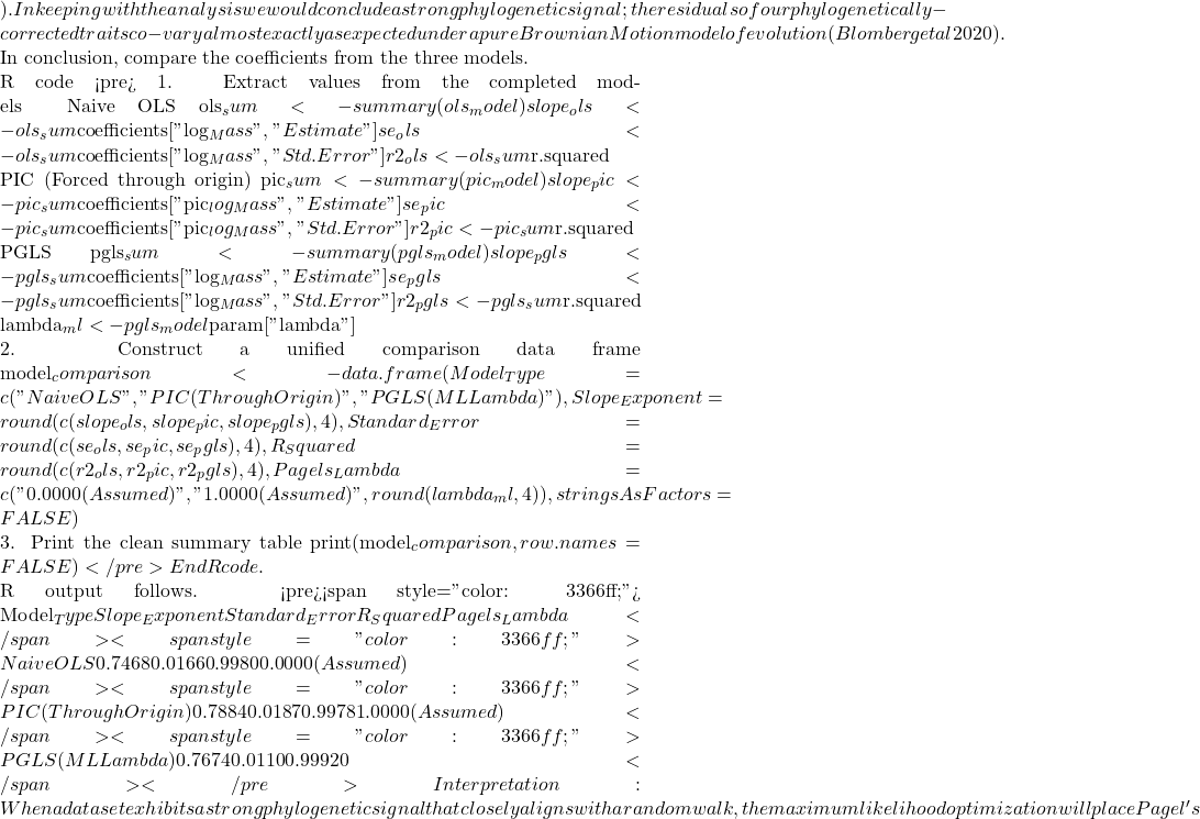 \lambda
 R^{2}$ values match identically between those two rows, while the naive OLS model stands apart due to its complete omission of tree topology.
Looking closely at the comparison of coefficients from the different models, from 0.7468 to 0.7884, it would be natural to ask, “Why go through the trouble of building a tree if the final biological answer is practically identical?” And, note that OLS and PGLS are nearly the same! The short response is only the phylogenetically correct coefficient estimates are statistically valid, and larger data sets are unlikely to reveal such agreement.
The fact that the PGLS slope (0.7674) splits the difference between the naïve OLS (0.7468) and strict PIC (0.7884) shows that Pagel’s λ converged on an intermediate value between 0 and 1. Instead of completely erasing the tree or treating it as absolute truth, PGLS multiplied the off-diagonal elements of the covariance matrix by this fractional λ value. This flattens the evolutionary branches, shrinking the expected covariance between sister taxa.
The model recognized that closely related species share some ancestral drag, but also exhibit more independent divergence than a pure random walk would predict. In contrast, the other two models represent rigid statistical boundaries:
- Naive OLS forces λ = 0, entirely ignoring the tree topology to arrive at
0.7468. - Strict PIC forces λ = 1, assuming unscaled Brownian Motion.
Because it used the full branch lengths, it shifted the trajectory heavily to 0.7884. By optimizing to an intermediate λ, PGLS strikes a perfect compromise: it protects us from the pseudoreplication of OLS while preventing the over-correction of a forced PIC.
Questions
- Mathematically, under what specific evolutionary conditions does a PGLS regression yield the exact same slope and standard error as a PIC regression?
- If your model estimates an optimized λ = 0.45, how does this physically alter the off-diagonal elements of your variance-covariance matrix compared to a standard OLS matrix?
- Why must a linear regression using Phylogenetically Independent Contrasts (PIC) be forced through the origin, omitting the standard intercept term?
- How does a PGLS matrix mathematically downweight a tight cluster of closely related species to prevent them from artificially inflating your sample size (N)?
- What happens to your Type I error rate and standard errors if you run a PGLS assuming Brownian Motion (λ = 1), but the trait actually evolved under strong stabilizing selection?
Explore on your own.
Kleiber’s data set (Table 2, 1947) contained data for humans (women) and four additional species. Redo the PIC and PGLS analysis with the updated data set. What is the effect on coefficient estimates and the standard errors with the (slightly) larger data set?
kleiber_full <- data.frame(
    Species = c("Mouse", "Rat", "Rabbit", "Macaque", "Cat", "Dog",
              "Goat", "Sheep", "Chimpanzee", "Woman", "Cow"),
# Exact body mass (W) in kilograms
    Mass = c(0.021, 0.282, 2.45, 4.20, 3.10, 13.40,
           36.00, 46.40, 38.00, 56.10, 439.00),
# Exact basal metabolic rate in kcal per 24 hours
    BMR = c(3.38, 32.7, 134.0, 207.0, 151.0, 506.0,
          826.0, 1145.0, 1090.0, 1398.0, 6135.0),
stringsAsFactors = FALSE
)
and the tree
"(((((Mouse:10,Rat:10):10,Rabbit:20):20,((Macaque:25,(Chimpanzee:6,Woman:6):19):10):10):10,(Cat:20,Dog:20):30):10,(Goat:15,Sheep:15):40,Cow:55);"
my_tree <- read.tree(text = expanded_newick)
References and suggested readings
Adams, D. C., & Collyer, M. L. (2019). Phylogenetic comparative methods and the evolution of Multivariate Phenotypes. Annual Review of Ecology, Evolution, and Systematics, 50(1):405–425.
Attwood, S. W., Hill, S. C., Aanensen, D. M., Connor, T. R., & Pybus, O. G. (2022). Phylogenetic and phylodynamic approaches to understanding and combating the early SARS-CoV-2 pandemic. Nature Reviews Genetics, 23(9), 547–562.
Blomberg, S. P., Rathnayake, S. I., & Moreau, C. M. (2020). Beyond Brownian Motion and the Ornstein-Uhlenbeck Process: Stochastic Diffusion Models for the Evolution of Quantitative Characters. American Naturalist, 195(2), 145–165.
Cornwallis, C. K., & Griffin, A. S. (2024). A guided tour of phylogenetic comparative methods for studying trait evolution. Annual Review of Ecology, Evolution, and Systematics, 55(1), 181–204.
Felsenstein, J (1985) Phylogenies and the comparative method. American Naturalist 125(1):1-15.
Felsenstein, J. (1988) Phylogenies and quantitative characters. Annual Review of Ecology and Systematics, 19, 445–471.
Garland Jr, T., Bennett, A. F., & Rezende, E. L. (2005). Phylogenetic approaches in comparative physiology. Journal of experimental Biology, 208(16), 3015-3035.
Grafen, A. (1989). The phylogenetic regression. Phil. Trans. R. Soc. London B, 326, 119-157.
Harvey, P.H. and Pagel, M.D. (1991) The Comparative Method in Evolutionary Biology. Oxford University Press, Oxford, Oxford Series in Ecology and Evolution.
Housworth, E. A., Martins, E. A. P., & Lynch, M. (2004). The phylogenetic mixed model. American Naturalist, 163, 84–96.
Kozłowski, J., & Konarzewski, M. (2004). Is West, Brown and Enquist’s model of allometric scaling mathematically correct and biologically relevant? Functional Ecology, 18(2), 283–289.
Martins, E.P. (1996) Phylogenies and the Comparative Method in Animal Behavior. Oxford University Press.
Mazel, F., Davies, T. J., Georges, D., Lavergne, S., Thuiller, W., & Peres-Neto, P. R. (2016). Improving phylogenetic regression under complex evolutionary models. Ecology, 97(2), 286–293.
Pagel, M. (1999). Inferring the historical patterns of biological evolution. Nature</i<, 401(6756), 877–884.
Paradis, E. (2012) Analysis of Phylogenetics and Evolution with R (Second Edition). New York: Springer.
Paradis, E. and Schliep, K. (2019) ape 5.0: an environment for modern phylogenetics and evolutionary analyses in R. Bioinformatics, 35, 526–528.
Pearse, W. D., Davies, T. J., & Wolkovich, E. M. (2025). How to Define, Use, and Interpret Pagel’s \ łambda \ (Lambda) in Ecology and Evolution. Global Ecology and Biogeography, 34(4), e70012.
Revell, L. J. (2012) phytools: An R package for phylogenetic comparative biology (and other things). Methods in Ecology and Evolution, 3, 217-223.
Rohlf, F. J. (2001). Comparative methods for the analysis of continuous variables: Geometric interpretations. Evolution, 55(11), 2143–2160.
Uyeda, J. C., Zenil-Ferguson, R., & Pennell, M. W. (2018). Rethinking phylogenetic comparative methods. Systematic Biology, 67(6), 1091-1109.
Zhang, J., Pei, N., & Mi, X. (2012). phylotools: Phylogenetic tools for Eco-phylogenetics. R package version 0.1, 2.
Chapter 20 contents
- Additional topics
- Area under the curve
- Peak detection
- Baseline correction
- Surveys
- Time series
- Dimensional analysis
- Estimating population size
- Diversity indexes
- Survival analysis
- Growth equations and dose response calculations
- Plot a Newick tree
- Phylogenetically independent contrasts
- How to get the distances from a distance tree
- Binary classification
- Meta-analysis
20.11 – Plot a Newick tree
Introduction
The phrase “paradigm shift”, attributed to Kuhn (1962, see Wikipedia), may be well-worn and even abused today (Naughton 2012), but the shift in thinking from essential types and group thinking (essentialism) to viewing species as varying individuals in populations (populating thinking) revolutionized biology (O’Hara 1997, Sandvik 2008). Tree thinking is the manifestation of Charles Darwin’s “descent with modification” metaphor (Gregory 2008). Thus, every biology student should have ability to work with, and interpret, phylogenetic trees (tree thinking). The subject of creating and working with phylogenetic graphs is complicated with an extensive library. A good review is available from Holder and Lewis (2003) and readers should know Felsenstein’s book (2004).
Here, I include a modest, incomplete primer on working with trees in R.
- Loading the tree file
- Change tip names
- Write tip names to a text file
- Plot the tree as phylogram or cladogram
- Get node labels
- Re-root the tree
- Write a tree to a file
I assume that the student already has a set of species or other taxa, gathered sequences (DNA or protein), aligned the sequences, estimated gene or phylogeny tree, and wishes to view and manipulate the tree in R. While these kinds of analyses can be done with R and R packages (see Task view: Phylogenetics), other software may be better choice for the student just beginning with phylogenetic tree building (see Unipro UGENE and MEGA, for examples). If the goal is just to view a tree file, or add annotations, then I recommend the iTOL tools.
Data formats
Phylogeny and gene trees are special cases of network graphs. Newick format (Wikipedia) is a common but limited representation of the tree which uses parentheses (groupings) and commas (branching). Other formats permit additional information; examples are Nexus file (Wikipedia) and the extension of Nexus to XML, NeXML (Wikipedia), and phyloXML (Wikipedia) formats. Our example uses Newick format.
Data set
I’ll use a “time tree” for an example. Tree from timetree.org, list of species (copy/paste list to a text file, load the text file Load list of of Species, then save the tree as a Newick file).
Alligator mississippiensis
Felis catus
Bos taurus
Gallus gallus
Pan troglodytes
Canis lupus
Homo sapiens
Anolis carolinensis
Macaca mulatta
Mus musculus
Didelphis virginiana
Sus scrofa
Oryctolagus cuniculus
Rattus norvegicus
R code
Requires the ape package. Phylotools and Phytools packages provide additional handy functions. References for these packages are listed at the end of this page.
require(ape)
require(phytools)
require(phylotools)
#If tree file, then
read.tree(file="tree14.nwk")
or
tree14 <- read.tree(file.choose())
#If no tree file saved, copy the Newick data use text="", replace example tree with your Newick tree
tree14 <-read.tree(text="((Anolis_carolinensis:279.65697667,(Gallus_gallus:236.50266286,Alligator_mississippiensis:236.50266286)'14':43.15431381)'13':32.24694470,(Didelphis_virginiana:158.59758758,(((Felis_catus:54.32144118,Canis_lupus:54.32144118)'11':23.43351523,(Bos_taurus:61.96598852,Sus_scrofa:61.96598852)'10':15.78896789)'19':18.70743276,((Oryctolagus_cuniculus:82.14079889,(Rattus_norvegicus:20.88741740,Mus_musculus:20.88741740)'9':61.25338149)'22':7.68238853,(Macaca_mulatta:29.44154682,(Pan_troglodytes:6.65090500,Homo_sapiens:6.65090500)'8':22.79064182)'6':60.38164060)'30':6.63920175)'29':62.13519841)'27':153.30633379);")
#return information about the object
tree14
Output returned by R
Phylogenetic tree with 14 tips and 13 internal nodes.
Tip labels:
Anolis_carolinensis, Gallus_gallus, Alligator_mississippiensis, Didelphis_virginiana, Felis_catus, Canis_lupus, ...
Node labels:
, 13, 14, 27, 29, 19, ...
Rooted; includes branch lengths.
Change the tip names. Create a data frame with the tip labels and new tip names.
require(phylotools)
timeTreeTips <- tree14$tip.label
replaceTips <- c("Alligator", "Cat", "Chicken", "Chimpanzee", "Cow", "Dog", "Human", "Lizard", "Macaque", "Mouse", "Opossum", "Pig", "Rabbit", "Rat")
myDat <- data.frame(timeTreeTips,replaceTips)
ntree14<- sub.taxa.label(tree14,myDat)
Collect and write the tip names to a text file
#Extract tips from newick file, write to text file
require(ape)
my.tips <- sort(tree14$tip.label)
#option 1
cat(my.tips,file="outfile.txt",sep="\n")
#option 2
my_conn = file("outfile.txt")
writeLines(my.tips,my_conn)
close(my_conn)
Next, make the plot.
plot(ntree14)
Result, a simple phylogram, i.e., a tree diagram with branching patterns and branch lengths proportional to amount of character change.
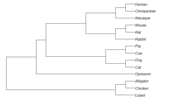
Figure 1. Phylogram plot of 14 taxa
Or, change from default “phylogram” to “cladogram” view.
plot(tree14, type="cladogram")
Figure 2. Cladogram view, same 14 taxa.
Note that while the tree is rooted, it’s a midpoint rooting, the default setting in Newick files. For true root based on outgroup(s), identify the nodes, then select root.
Add node labels; plot() must be run first.
nodelabels()
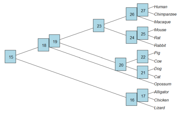
Figure 3. Plot of tree with labeled nodes.
The outgroup(s) were the reptiles (Alligator, Chicken, Lizard), so reroot at node 16.
rrTree<- root(tree14, node=16)
plot(rrTree, type="cladogram")
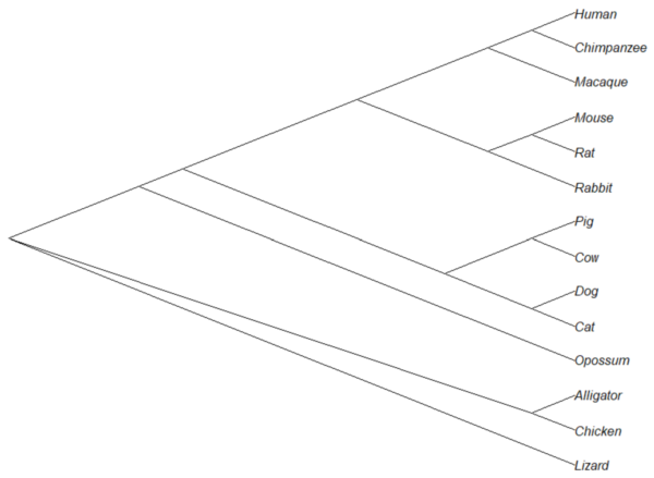
Figure 4. Re-rooted tree.
Write tree to a file
require(ape)
To export tree to Newick format
write.tree(tree14, file = "filename.nwk")
for Nexus format
write.nexus(tree14, file = "filename.nex")
Star phylogeny
Collapse the tree to a star phylogeny, an unlikely evolutionary model in which the species resulted from “… a single explosive adaptive radiation” (Felsenstein 1985). Star phylogeny is an extreme tree shape, or multifurcation (polytomy), where all tips derive from the same node (Colijn and Plazzotta 2018). This type of phylogeny can be viewed as a null model for inference (but see Bayesian “star phylogeny paradox,” cf. Kolaczkowski and Thornton 2006).
require(phytools)
ctree14 <-collapse.to.star(tree14, 15)
plot(ctree14, type="cladogram")
Figure 5. Star phylogeny
Under a star phylogeny model, all taxa are assumed independent of each other, in contrast to the nested hierarchical model of evolution (e.g., Fig. 4), which shows a lack of independence among the taxa. More succinctly, a fitted to uncorrected taxa comparisons may violated the assumption that errors are independent and identically distributed. Phylogenetically correct methods attempt to address the lack of independence among taxa for comparative analysis (Felsenstein 1985, Uyeda et al 2016). Biologists should know about Felsenstein’s 1985 paper. Felsenstein’s paper created a paradigm shift in how to analyze comparative datasets and has been cited more than ten thousand times (1 August 2023, Google Scholar). To put that number in context, the 1986 paper by Kary Mullis et al., which announced invention of PCR with thermally stable polymerase that has revolutionized molecular biology, has been cited 6721 times over that same period.
Additional packages of note
The R package tanggle works with the package ggtree and advantage of the ggplot2 environment. Contains many functions to work with phylogeny graphs including re-rooting and swapping nodes. The package is available from Bioconductor,
if (!requireNamespace("BiocManager", quietly = TRUE))
    install.packages("BiocManager")

BiocManager::install("tanggle")
ggtree is also a Bioconductor package, not available at CRAN.
Online viewers
Many browser-based tree viewers online, including icytree.org and iTOL tools. Additional tree viewers listed at Wikipedia.
References and suggested readings
Colijn C, Plazzotta G. A Metric on Phylogenetic Tree Shapes. Syst Biol. 2018 Jan 1;67(1):113-126.
Felsenstein, J (1985) Phylogenies and the comparative method. American Naturalist 125(1):1-15.
Felsenstein, J. (2004). Inferring phylogenies. Sunderland, MA: Sinauer associates.
Gregory, T. R. (2008). Understanding evolutionary trees. Evolution: Education and Outreach, 1(2), 121-137.
Holder, M., & Lewis, P. O. (2003). Phylogeny estimation: traditional and Bayesian approaches. Nature reviews genetics, 4(4), 275-284.
Kuhn, T. S. (1962). The structure of scientific revolutions. University of Chicago Press: Chicago.
Mullis, K., Faloona, F., Scharf, S., Saiki, R. K., Horn, G. T., & Erlich, H. (1986, January). Specific enzymatic amplification of DNA in vitro: the polymerase chain reaction. In Cold Spring Harbor symposia on quantitative biology (Vol. 51, pp. 263-273). Cold Spring Harbor Laboratory Press.
Naughton, J. (2012, August 18). Thomas Kuhn: The man who changed the way the world looked at science. The Guardian. https://www.theguardian.com/science/2012/aug/19/thomas-kuhn-structure-scientific-revolutions
O’Hara, R. J. (1997). Population thinking and tree thinking in systematics. Zoologica scripta, 26(4), 323-329.
Paradis, E. (2012) Analysis of Phylogenetics and Evolution with R (Second Edition). New York: Springer.
Paradis, E. and Schliep, K. (2019) ape 5.0: an environment for modern phylogenetics and evolutionary analyses in R. Bioinformatics, 35, 526–528.
Revell, L. J. (2012) phytools: An R package for phylogenetic comparative biology (and other things). Methods in Ecology and Evolution, 3, 217-223.
Sandvik, H. (2008). Tree thinking cannot taken for granted: challenges for teaching phylogenetics. Theory in Biosciences, 127(1), 45-51.
Uyeda, J. C., Zenil-Ferguson, R., & Pennell, M. W. (2018). Rethinking phylogenetic comparative methods. Systematic Biology, 67(6), 1091-1109.
Zhang, J., Pei, N., & Mi, X. (2012). phylotools: Phylogenetic tools for Eco-phylogenetics. R package version 0.1, 2.
Chapter 20 contents
- Additional topics
- Area under the curve
- Peak detection
- Baseline correction
- Surveys
- Time series
- Dimensional analysis
- Estimating population size
- Diversity indexes
- Survival analysis
- Growth equations and dose response calculations
- Plot a Newick tree
- Phylogenetically independent contrasts
- How to get the distances from a distance tree
- Binary classification
- Meta-analysis
13.1 – ANOVA Assumptions
Introduction
Like all parametric tests, assumptions are made about the data in order to justify and trust estimates and inferences drawn from ANOVA. While acknowledging the “experimental design” message suggested by the xkcd panel in Figure 1 — the presence of a large effect size between groups mitigates the technical necessities of inferential statistics — of course, not all of our projects will have such obvious results. Understanding the impact of assumptions on inference is a key concept in (bio)statistics: when the p-value is close to the Type I error rate, deviations from assumptions may reduce our confidence in the “statistical significance” of the result.

Figure 1. xkcd.com “Statistics,” https://xkcd.com/2400/.
ANOVA assumptions include:
- Data come from normal distributed population. View with a histogram or Q-Q plot. Test with Shapiro-Wilks or other appropriate goodness of fit test (see Question 1 below). Normality tests are the subject of Chapter 13.3.
- Sample size equal among groups.
- This is an example of a potentially confounding factor — If sample sizes differ, then any difference in means could be simply because of differences in sample size! This gets us into weighted versus unweighted means.
- You shouldn’t be surprised that modern implementations of ANOVA in software easily handle (adjust for) these known confounding factors. Depending on the program, you’ll see “Adjusted means,” “least squares means,” “Marginal means” etc. This just implies that the group means are compared after accounting for confounding factors.
- Importantly, as long as sample sizes among the groups are roughly equivalent, normality assumption is not a big deal (low impact on risk of Type I error).
- Independence of errors. One consequence of this assumption is that you would not view 100 repeated observations of a trait on the same subject as 100 independent data points. We’ll return to this concept more in the next two lectures. Some examples:
-
- Colorimetric assay where the signal changes over time, and you measure in order (eg, samples from group 1 first, samples from group 2 second, etc.) — this confounds group with time.
- The consequence is that you are far more likely to reject the null hypothesis, committing a Type I error.
- Let’s say you are observing running speeds of ten mongoose. However, it turns out that five of your subjects are actually from the same family, identical quintuplets! Do you really have ten subjects?
- Compare brain-body mass ratio among different species; this is a classic comparative method problem (Fig 3). Since 1985 (Felsenstein 1985), it was recognized that the hierarchical evolutionary relationships among the species must be accounted for to control for lack of independence among the taxa tested. See Phylogenetically independent contrasts, Chapter 20.12.
- Colorimetric assay where the signal changes over time, and you measure in order (eg, samples from group 1 first, samples from group 2 second, etc.) — this confounds group with time.
- Equal variances (homogeneity) among groups. See Chapter 13.4 for how to test this for multiple groups.
Impact of assumptions
R — and pretty much all statistics packages — will calculate the ANOVA table and the p-value, but it is up to you to recognize that the P-value is accurate only if the assumptions are met. Violation of the assumption of normality can lead to Type I errors occurring more often than the 5% level. What to do if the assumptions are violated?
If the violation is due to only a handful of the data, you might proceed anyway. But following a significant test for normality, we could avoid the ANOVA in favor of nonparametric alternatives (Chapter 15), or, we might try to transform the data.
Consider a histogram of brains weight measures in grams for a variety of mammals (Fig 2).
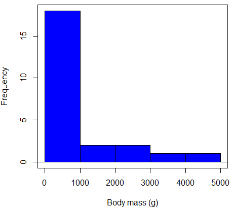
Figure 2. Histogram of body mass (g) for 24 mammals (data from Boddy et al 2012).
We will introduce a variety of statistical tests of the assumption of normality in Chapter 13.3, but looking at a histogram as part of our data exploration, we clearly see the data are right-skewed (Fig 2). Is this an example of normal distributed sample of observations? Clearly not. If we proceed with statistical tests on the raw data set, then we are more likely to commit a Type I error (ie, we will reject the null hypothesis more often than we should).
A comment on normality and biology. It is very possible that data may not be normally distributed or have equal variances on the original scale, but a simple mathematical manipulation may take care of that. In fact, in many case in biology that involve growth, many types of variables are expected to not be normal on the original scale. For example, while the relationship between body mass,  , and metabolic rate,
 , in many groups of organisms is allometric and increases positively, the relationship

is not directly proportional (linear) on the original scale. By taking the logarithm of both body mass and metabolic rate, however, the relationship is linear

In fact, taking the logarithm (base 10, base 2, or base e) is often a common solution to both non-normal data (Fig 2) and unequal variances.
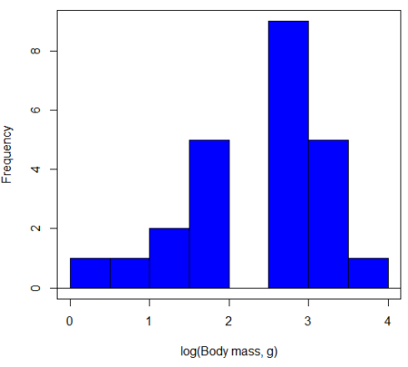
Figure 3. Histogram of log10-transformed body mass observations from Figure 2.
Other common transformations include taking the square root or the inverse of the square-root for skewed or kurtotic sample distributions, and the arcsine for frequencies (since frequencies can only be from 0 to 1 — need to “stretch the data” to make frequencies fit procedures like ANOVA). There are many issues about data transformation, but keep in mind three points. After completing the transformation, you should check the assumptions (normality, equal variances) again.
You may need to recode the data before applying a transform. For example, you cannot take the square root or logarithm of negative numbers. If you do not recode the data, then you will lose these observations in your subsequent analyses. In many cases, this problem is easily solved by adding 1 to all data points before making the transform. I prefer to make the minimum value 1 and go from there. The justification for data transformation is basically to realize that there is no necessity to use the common arithmetic or linear scale: many relationships are multiplicative or nonadditive (eg, rates in biology and medicine).
Note 1: Instead of transformations or other ad hoc manipulations of the data, modern statistical approaches favor modeling the error structure of the data within a Generalized Linear Model framework (St.-Pierre et al 2018). The advantage of the model approach is that parameter estimation occurs on the raw data. Use of transformations may, however, remain a better choice. While statistically justified, the generalized linear model approach may also tend to have higher rates of Type II error compared to simple transformations.
Statistical outlier
Another topic we should at least mention here is the concept of outliers. While most observations tend to cluster around the mean or middle of the sample distribution, occasionally one or more observations may differ substantially from the others. Such values are called outliers, and we note that there are two possible explanations for an outlier
- the value could be an error.
- it is a true value.
Note 2: “it is a true value,” and there may be an interesting biological explanation for its cause, ie, extraordinary individuals.
We encountered a clear outlier in the BMI homework. If the reason is (1), then we go back and either fix the error or delete it from the worksheet. If (2), however, then we have no objective reason to exclude the point from our analyses.
We worry if the outlier influences our conclusions — so it is a good idea to run your analyses with and without the outlier. If your conclusions remain the same, then no worries. If your conclusions change based on one observation, then this is problematic. For the most part you are then obligated to include the outlier and the more conservative interpretation of your statistical tests.
ANOVA is robust to modest deviations from assumptions
A comment about ANOVA assumptions ANOVA turns out to be robust to violations of item (1) or (2). That means unless the data are really skewed or the group sizes are very different, ANOVA will perform well (Type I error rate stays close to the specified 5% level). We worry about this however when p-value is very close to alpha!!
The third assumption is more important in ANOVA.
Like the t-test, ANOVA makes the assumption of equal variances among the groups, so it will be helpful to review why this assumption is important to both the t-test and ANOVA. In the two-sample independent t-test, the pooled sample variance,  , is taken as an estimate of the population variance,
 . If you recall,
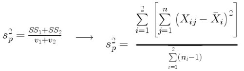
where  refers to the sum of squares for the first group and
 refers to the second group sum of squares (see our discussion on measures of dispersion) and
 refers to the degrees of freedom for the first group and
 refers to the second group degrees of freedom. We make a similar assumption in ANOVA. We assume that the variances for each sample are the same and therefore that they all estimate the population variance . To say it in another way, we are assuming that all of our samples have identical variability
Once we make this assumption, we may pool (or combine) all of the SSs and DFs for all groups as our best estimate of the population variance, . The trick to understanding ANOVA is to realize that there can be two types of variability: there is variability due to being part of a group (eg, even though ten human subjects receive the same calorie-restricted diet, not all ten will loose the same amount of weight) and there is variability among or between groups (eg, on average, all subjects who received the calorie-restricted diet lost more weight than did those subjects who were on the non-restricted diet).
Example
The encephalization index (or encephalization quotient) is defined as the ratio of size the brain compared to body size. While there is a well-recognized increase in brain size given increased body size, encephalization describes a shift of function to cortex (frontal, occipital, parietal, temporal) from noncortical parts of the brain (cerebellum, brainstem). Increased cortex is associated with increased complexity of brain function; for some researchers, the index is taken as a crude estimate of intelligence. Figure 4A shows plot of brain mass in grams versus body size (grams) for 24 mammal species (data sampled from Boddy et al 2012); Figure 4B shows the same data, but following log10-transform of both variables.
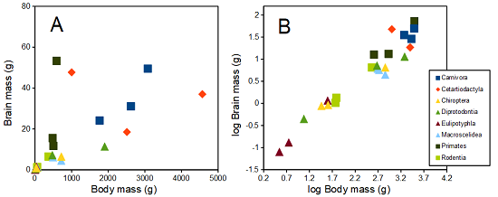
Figure 4. Plot of brain and body weights (A) and log10-log10 transform (B) for a variety of species (data from Boddy et al 2012). The ratio is called encephalization index.
Looking at the two figures the linear relationship between the two variables is obvious in Figure 4B, less so for Figure 4A. Thus, one biological justification for transformation of the raw data is exemplified with the brain-body mass dataset: the association is allometric not additive. The other reason to apply a transform is statistical; the log10-transform improves the normality of the variables. Take a look at the Q-Q plot for the raw data (Fig 5) and for the log10-transformed data (Fig 6).
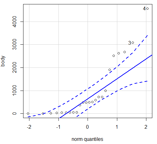
Figure 5. Q-Q plot, body mass, raw data. Compare to Figure 2.
Figure 5 is a good test of your observation skills — what are you supposed to look for in a Q-Q plot? Follow the dots — the data don’t fall on the straight line. A few even fall outside of the confidence interval (the curved dashed lines), which suggests the data were not normally distributed (see histogram, Fig 2). And for the transformed data, the Q-Q plot is shown in Figure 6.
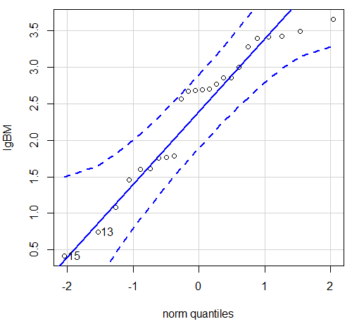
Figure 6. Q-Q plot same data, log10-transformed, compare to Figure 2.
Compared to the raw data, the transformed data now fall on the line and none are outside of the confidence interval. We would conclude that the transformed data are more normal, thus, better meeting the assumptions of our parametric tests.
Lack of independence among data
Species comparisons are common in evolutionary biology and related fields. As noted earlier, comparative data should not be treated as independent data points (discussed in 20.12 – Phylogenetically independent contrasts). For our 24 species, I plotted the estimate of the phylogeny (timetree.org), represented in Figure 7. Some species are closely related (eg the two elephant shrews, Rhynchocyon genus). Thus, because of the hierarchical, nested nature of evolution — first articulated by Charles Darwin — instead of 24 independent data points, we have eight clusters of points (see Question 4).
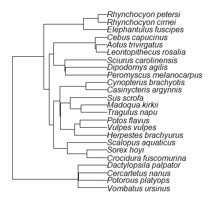
Figure 7. Phylogenetic tree of 24 species used in this report.
Note 3: The relevant quote from Charles Darwin: “… the inevitable result is that the modified descendants proceeding from one progenitor become broken up into groups subordinate to groups,” and was illustrated by the only figure in Origin of Species (both quote and illustration are in Chapter 4).
The conclusion? We don’t have 24 data points, more like 8 points. Because the species are more or less related, there are fewer than 24 independent data points. Statistically, this would mean that the errors are correlated. Various approaches to account for this lack of independence have been developed; perhaps the most common approach is to apply phylogenetically independent contrasts, a topic discussed in Chapter 20.12. (Boddy et al 2012 used this approach.)
Note 4: See 20.11 – Plot a Newick tree for how to plot phylogeny trees in R.
Questions
- Make a histogram for the brain mass data set.
- Shapiro-Wilks is one test of normality.
- Can you recall the name of the other normality tests we named?
- Run tests of normality on both body mass and brain mass data. Interpret the results, frame your response with keywords: “central tendency,” “outliers,” “shape,” and “symmetry.”
- Calculate moment statistics for the body mass and brain mass data set, both raw and log10-transformed data. Interpret your results, taking care to frame your answer with the following keywords: “shape,” “symmetry,” and “peakedness” (aka “tailedness”).
- We introduced the lack of independence for comparative data attributed to the evolutionary process. Statistically, the impact is on degrees of freedom; for example, if we ignore the lack of independence in the data set, df = 22 for the slope coefficient in a linear regression. However, given the degrees of freedom would be closer to six! What are the effects on Type I error rate of lack of independence?
Quiz Chapter 13.1
ANOVA assumptions
Data set and R code used in this page
species, order, body, brain
'Herpestes ichneumon', Carnivora, 1764, 24.1
'Potos flavus', Carnivora, 2620, 31.05
'Vulpes vulpes', Carnivora, 3080, 49.5
'Madoqua kirkii', Cetartiodactyla, 4570, 37
'Sus scrofa', Cetartiodactyla, 1000, 47.7
'Tragulus napu', Cetartiodactyla, 2510, 18.5
'Casinycteris argynnis', Chiroptera, 40.5, 0.92
'Cynopterus brachyotis', Chiroptera, 29, 0.88
'Potorous platyops', Chiroptera, 718, 6.5
'Cercartetus nanus', Diprotodontia, 12, 0.44548
'Dactylopsila palpator', Diprotodontia, 474, 7.15876
'Vombatus ursinus', Diprotodontia, 1902, 11.396
'Crocidura fuscomurina', Eulipotyphla, 5.6, 0.13
'Scalopus aquaticus', Eulipotyphla, 39.6, 1.48
'Sorex hoyi', Eulipotyphla, 2.6, 0.107
'Elephantulus fuscipes', Macroscelidea, 57, 1.33
'Rhynchocyon cirnei', Macroscelidea, 490, 6.1
'Rhynchocyon petersi', Macroscelidea, 717.3, 4.46
'Aotus trivirgatus', Primates, 480, 15.5
'Cebus capucinus', Primates, 590, 53.28
'Leontopithecus rosalia', Primates, 502.5, 11.7
'Dipodomys agilis', Rodentia, 61.4, 1.34
'Peromyscus melanocarpus', Rodentia, 58.8, 1.03
'Sciurus carolinensis', Rodentia, 367, 6.49
The Newick code for the tree in Figure 6.
((Vombatus_ursinus:48.94499077,((Potorous_platyops:47.59556667,Cercartetus_nanus:47.59556667)'14':0.66887333,Dactylopsila_palpator:48.26444000)'13':0.68055077)'11':109.65259681,(((((Crocidura_fuscomurina:33.74066667,Sorex_hoyi:33.74066667)'10':33.03022424,Scalopus_aquaticus:66.77089091)'19':22.55292749,(((Herpestes_brachyurus:54.32144118,(Vulpes_vulpes:45.52834967,Potos_flavus:45.52834967)'9':8.79309151)'22':23.43351523,((Tragulus_napu:43.96862857,Madoqua_kirkii:43.96862857)'8':17.99735995,Sus_scrofa:61.96598852)'6':15.78896789)'30':0.77378567,(Casinycteris_argynnis:35.20000000,Cynopterus_brachyotis:35.20000000)'29':43.32874208)'27':10.79507632)'35':7.13857077,(((Peromyscus_melanocarpus:69.89837667,Dipodomys_agilis:69.89837667)'43':0.64655123,Sciurus_carolinensis:70.54492789)'42':19.27825952,((Leontopithecus_rosalia:18.38385647,Aotus_trivirgatus:18.38385647)'40':1.29720005,Cebus_capucinus:19.68105652)'48':70.14213090)'51':6.63920175)'47':8.99739162,(Elephantulus_fuscipes:39.23366667,(Rhynchocyon_cirnei:15.34500000,Rhynchocyon_petersi:15.34500000)'39':23.88866667)'56':66.22611412)'55':53.13780679);