14.2 – Sources of variation
Introduction
Sources of variation, or components of the two-way ANOVA include two factors, each with two or more levels (groups), and collectively, factors are often referred to as the main effects in these types of ANOVA. The other source of variation in a two-way ANOVA is the interaction between the two factors. Below, I have listed the important components, although I have not included how the sum of squares are calculated. You are expected to know the sources of variation for this most basic two-way ANOVA table (Fig. 1). You should also be able to solve any missing elements in one of these tables by utilizing any included information.
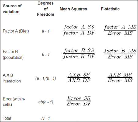
Figure 1. ANOVA table for two-way, balanced, replicated design.
Taking each row from Figure 1 one at a time we have
| Source | DF | Mean Squares | F-statistic |
| First Factor |  |
 |
 |
where Source refers to the source of variation, DF refers to Degrees of Freedom, a is the number of levels (groups) of the first factor, SS refers to Sum of Squares, and MS refers to the Mean Squares.
Next is the second factor
| Source | DF | Mean Squares | F-statistic |
| First Factor |  |
 |
 |
where b is the number of levels (groups) of the second factor. Next is the interaction between the first and second factors.
| Source | DF | Mean Squares | F-statistic |
| Interaction |  |
 |
 |
and lastly the Within-cell Error or residual source of variation
| Source | DF | Mean Squares | F-statistic |
| Error |  |
 |
 |
where n is the number of experimental units for each group. Note that if the sample size differs for one or more groups (levels),then the design would be unbalanced and this formula does not work to determine the degrees of freedom. The total degrees of freedom for the two-way ANOVA is simply N – 1, where N is the sample size for the entire problem; a little algebra shows that N may be calculated as

Unbalanced designs
An unbalanced design implies that observations are missing value for one or more groups. What to do if data are missing? Decision depends on how the data are missing (see Chapter 5). For example, if data are missing at random with respect to treatment, then this should not affect inference. If data are missing not at random, then inference, logically, must be impacted. Calculating the ANOVA, moreover, becomes a different matter. In the one-way ANOVA, no real problem arises although setting up contrasts among the levels requires a weighting term to be factored into the calculations. For higher-level ANOVA involving two or more factors the sums of squares for treatment effects are no longer simple partitioning into the different sources of variation. The sources overlap and the order by which the Factors enter into the statistical model now affects the calculations. Thus, while setting up the calculations for the balanced design is straight-forward, perhaps surprisingly, if group sizes differ, this simple relationship for calculating the degrees of freedom, sums of squares, and Mean squares become an unsolvable problem. This problem is largely solved by the general linear model.
Questions
- Based on the results of a two-way ANOVA, the error sums of squares (SSE) was computed to be 160. If we ignore one of the factors and perform a one-way ANOVA using the same data, will the SSE be the same as in the two-way ANOVA, or will it increase? Decrease? Explain your choice.
- While conducting a two-way ANOVA, you conclude that a statistically significant interaction exists between factor 1 and factor 2. What should be your next step? Do you drop the interaction term from the model and redo the analysis or do you report the results of factor effects including the non-significant interaction?
Quiz Chapter 14.2
Sources of variation
Chapter 14 contents
14 – ANOVA designs, multiple factors
Introduction
In our previous discussions about t-tests and ANOVA we focused on procedures with one dependent (response) variable and a single independent (predictor) factor variable that may cause variation in the response variable. In this chapter we extend our discussions about the general linear model by reviewing
- One-way ANOVA and provided a few examples of the one-way design.
- To review and set the stage for adding a second independent variable to the model.
Additional one-way ANOVA examples
1. In a plants, we may have a response variable like height and one factor variable (location: sun vs. shade) thought to influence plant height (eg, Aphalo et al 1999).
2. Pulmonary macrophage phagocytosis behavior (response variable) after exposure of toads to clean air or ozone (factor with 2 levels) (Dohm et al. 2005).
3. Monitor weight change on subjects after 6 weeks eating different diet (DASH, control) (Elmer et al. 2006).
All three of the examples are based on the same statistical model which may be written as:

where μ is the grand mean, Y is the response variable and A is the independent variable, or factor, with k = 1, 2, …. K levels, groups, or treatments. The total number of experimental units (eg, subjects) is given by i = 1, 2, 3, … n. Note that in the first and third examples, because there were only two groups (example 1: k = location, shade; example 3: k = DASH, control) note that this problem could have been evaluated as an independent sample t-test. For the second example, there were three groups so k = clean air, first ozone level, second ozone level).
Two-way ANOVA with replication
As useful as the one-way ANOVA design can be, it is a “one-factor-at-a-time” approach (Radzilani et al 2025), experiments are typically more complicated than a single t-test or one-way ANOVA design can handle; rarely would we conduct an experiment that reflects only one source of variation. Looking only at variability for one factor at a time while while keeping all other factors constant ignores interactions between factors, resulting in potentially serious model bias (eg, discussed in Vatcheva et al 2015).
For example, while diet has a profound effect on weight, clearly, activity levels are also important. At a minimum, when considering a weight loss program, we would want to control or monitor activity of the subjects. This is a two-factor model, and the main effects, the two factors, were diet (factor A) and activity, (factor B). Both are expected to affect weight loss, and, perhaps, they may do so in complicated ways — an interaction (eg, on DASH diet, weight loss is accelerated when subjects exercise regularly).

The subject of this chapter is the introduction to two-way ANOVA designs. In fact, to many, ANOVA design is practically synonymous to a statistician when they think about experimental design (Lindman 1992; Quinn and Keough 2002). As noted by Quinn and Keough (2002) in the preface to their book, “… many biological hypotheses, even deceptively simple ones, are matched by complex statistical models” (p. xv). Once you start adding factor variables there becomes a number of ways in which the groups and experimental units can be distributed, and thus impact the inferences one can make from the ANOVA results. The first statistical model we introduced was the one-way ANOVA. Next, we begin the two-way ANOVA with the crossed, balanced, fully replicated design. Along the way we introduce model symbols to help us communicate the design structure and implications of the statistical models.
Quizzes in this chapter
A total of 71 questions among the several subchapters, a mix of true or false and multiple choice question format.