20.14 – Binary classification
draft
Introduction
For much of this textbook we emphasized the search for causal explanations — applied (bio)statistics. Machine learning refers to any system used that churns data into predictions, while not necessarily explaining how the collection of predictors effect the outcome (Li and Tong 2022).
Classification in science is the act of grouping observations based on common features. In data science, classification procedures are used to predict which category a data point belongs to by finding the lines or planes — the decision boundary — that best divide the different classes.
Prediction or decision – use data to build or “train” a model that is then used to make future predictions or decisions given new data. Technically, prediction and decision are different concepts — prediction refers to what might happen given new information while decision is about what we may do given new information. We discussed prediction as a goal of regression models in some detail in Chapter 17 and Chapter 18.
Linear discriminant analysis (LDA) is a well known classification algorithm, whose roots trace back to R.A. Fisher. Linear discriminant analysis finds a linear combination of features that characterizes or separates two or more classes of objects or events. It builds on the idea of multiple linear regression: for multiple linear regression we predict a continuous outcome variable from a set of predictor variables; for discriminant analysis, we predict discrete outcomes, two or more mutually exclusive groups, from a set of predictor variables.
Logistic regression (LR) is another common classification algorithm. We previously introduced LR as a statistical method for modeling the dependence of a binomial outcome variable on one or more categorical or continuous predictor variables (see Chapter 18.3 – Logistic regression). LR shares many features with linear discriminant analysis, but while LDA models the distribution of the data and assumes normality for the predictor variables, LR directly models the probability of the outcome, making fewer assumptions about the distribution of the data. LDA returns a discriminant function, a linear combination of the features, while LR returns a probability between 0 and 1 via the logistic function, estimating the probability of the data point belonging to a specific class.
Both LDA and LR return single decision models — not the same classification model, of course. The downside for use of a single model to predict based on new data is that the assumptions used to build the model may not hold for the new data. Enter learning methods like random forest. Random forest is an example of supervised learning methods — it combines the predictions of multiple models to get a better result than any single model could achieve alone. The idea is that a “forest” of multiple decision trees are generated, trained on different subsets of data, which then contribute towards a classification choice based on the consensus of those many decision trees. By “training the model” in machine learning we imply a process by which we help an algorithm to recognize patterns in data to make predictions on new, unseen data. Model parameters are learned from the data during training, hyperparameters are settings that control the model training process.
Note 1: Supervised learning implies we use “labeled” data, where we already know to which group outcomes belong. Unsupervised learning uses unlabeled data to find hidden patterns or structures within the data.
R packages
caret — a “comprehensive package” for training and tuning predictive models. “Tuning” refers to optimizing the performance of a model by adjusting its hyperparameters.
ranger — for building random forest model of classification and regression models.
Questions
pending
Quiz
pending
References and suggested readings
Blei, D. M., & Smyth, P. (2017). Science and data science. Proceedings of the National Academy of Sciences, 114(33), 8689–8692.
Boehmke, B., & Greenwell, B. N. (2019). Hands-On Machine Learning with R. Chapman and Hall/CRC. https://bradleyboehmke.github.io/HOML/
Bzdok, D., Altman, N., & Krzywinski, M. (2018). Statistics versus machine learning. Nature Methods, 15(4), 233–234.
Hastie, T., Tibshirani, R., & Friedman, J. (2009). The Elements of Statistical Learning: Data Mining, Inference, and Prediction (2nd ed.). Springer.
Li, J. J., & Tong, X. (2020). Statistical hypothesis testing versus machine learning binary classification: Distinctions and guidelines. Patterns, 1(7).
Lin, X., Cai, T., Donoho, D., Fu, H., Ke, T., Jin, J., Meng, X.-L., Qu, A., Shi, C., Song, P., Sun, Q., Wang, W., Wu, H., Yu, B., Zhang, H., Zheng, T., Zhou, H., Zhou, J., Zhu, H., & Zhu, J. (2025). Statistics and AI: A Fireside Conversation. Harvard Data Science Review, 7(2).
Chapter 20 contents
- Additional topics
- Area under the curve
- Peak detection
- Baseline correction
- Surveys
- Time series
- Dimensional analysis
- Estimating population size
- Diversity indexes
- Survival analysis
- Growth equations and dose response calculations
- Plot a Newick tree
- Phylogenetically independent contrasts
- How to get the distances from a distance tree
- Binary classification
- Meta-analysis
2.1 – Why (Bio)Statistics?
- What are the basic elements of biostatistics? .
- Why we require you to take Biostatistics as part of your major?.
- But, I’m pre-med and plan to apply to medical school ….
- With machine learning and AI, why learn biostatistics?.
- In what disciplines are biostatisticians employed?.
- Conclusions.
- Questions.
- Quiz.
- Chapter 2 contents
What are the basic elements of biostatistics?
.
What will you learn from an introductory course on (bio)statistics? Concepts and skills: An understanding (concepts) about the purpose and limits of descriptive statistics, inferential statistics, and statistical modeling for answering questions in biology and how to use elements of R programming (skills) applied to biology-related data sets to accomplish these tasks (see Table 1). Related, you will learn how (skills) to collect and manage data from projects, and why (concepts) statistical analysis can help answer questions, even inform decisions in public health. Thus, assessment in BI-311 of student learning includes both formative and summative assignments, exams, and culminates with a student research project.
Note 1: From time to time in this book I write “(bio)statistics” instead of “biostatistics.” It’s my subtle way of highlighting that whatever argument or statement is attached applies more generally to the statistical discipline, not just biostatistics. However, I’m not particularly consistent with this typology in the book.
What skills are you going to get from all of this? You will get different opinions on the elements of an essential first course in statistics or biostatistics. Certainly the basics are a foundation in probability and a breadth of classical elementary statistical procedures, which will include descriptive statistics, analysis of variance and linear regression, and an introduction to multivariate analysis. In preparation for your course in epidemiology you will also be introduced to risk analysis and survival analysis. However, the primary return for your time, I hope, will be a deeper appreciation for how to think about problems in biology from experimental design and data analysis perspectives. Practical skills you will learn include how to process and clean data for analysis, data visualization, and a foundation in parametric and nonparametric statistical methods.
The data sets described and provided in this course are small, with sample sizes in the tens to thousands (rarely). This framework is consistent with the development of the discipline of (bio)statistics, which originated to help interpret experiments conducted in agriculture, industry, and medical research (see Chapter 2.3). But, as you now know, because of genomics and other data-intensive disciplines, data sets can be very large, much beyond the kinds of data sets used prior to use of the computer in data analysis. However, as we will argue later on this page, learning foundational skills in (bio)statistics with small data sets facilitates working with and gaining insights from larger data sets. For example, we will emphasize during our work this semester how to develop a workflow with small data sets; these same workflows then can be scaled up and would include pipelines — based on tools and techniques developed in the broader discipline of bioinformatics — to large data sets, including use of Artificial Intelligence and machine learning.
Note 2: In data science, a workflow refers to the entire, end-to-end process needed in a project, from data collection, data processing, to descriptive statistics and modeling or inferential statistics, and report writing. A pipeline described elements of a workflow that can be automated.
Why we require you to take (Bio)statistics as part of your major?
.
At Chaminade University we require all biology students to take biostatistics, and we do so with an emphasis on use of data analysis skill development. This requirement aligns our program to national expectations of biology undergraduate education (eg, AAAS, NAS, NIH, NSF). As stated in Bio2010: Transforming Undergraduate Education for Future Research Biologists,
“Biology majors should be adept at using computers to acquire and process data, carry out statistical characterization of the data and perform statistical tests, and graphically display data in a variety of representations (p. 15).”
Learning biostatistics from a course like BI311 — which relies heavily on use of the R programming language and data sets — helps the biology student develop these skills.
In the next pages I will outline a history of statistics (Chapter 2.3), but here I wish to make the point that biostatistics is now considered to be a core skill set for biologists. Biostatistics as a discipline came into its own in the 1930’s, but extensive reliance on statistics in research really dates to more recent times because of the ubiquity of personal computers (Salsburg 2002). Modern biological and biomedical research requires computational and quantitative methods to collect, process, analyze, and interpret large data sets. And yet, even a casual survey of required courses for entry into graduate programs in biology (eg, only recommended for admissions to Marine Biology and Cell and Molecular Biology programs at University of Hawaiʻi – Manoa) will reveal that biostatistics is not required of candidates; so, what gives?
The first point is that programs list only minimum requirements. The second point is that many programs (genomics, ecology, etc) will expect the graduate student to take a year or more of (bio)statistics. The need is so crucial that at Harvard Medical School, all biology graduate students are expected to take a crash-course in computing and statistics to work with data (Stefan et al 2015).
Moreover, while graduate programs are not listing statistics as a requirement, many biology undergraduate curricula now require a course in (bio)statistics to reflect the increasingly data driven modern biology — where the jobs are!
My BI-311 students, I’ll make you a bet — or at least, I’ll make this part of your required homework (see BI311 Workbook)! Even a causal search of a research journal article in a biology discipline of your choosing will prove that there is no doing biology research today without an understanding of statistics.
But, I’m pre-med and plan to apply to medical school …
.
Even a cursory look at the literature will result in finding many authors strongly calling for this kind of preparation for a successful career in medicine (eg, Brieger and Hardin 2012). It’s obvious, but needs stating — you’re applying to medical school to become a doctor — you’ll spend the majority of your adult life as a doctor. Statistical thinking is crucial to answering the daily question: “My patient tested positive for biomarker X, what’s the chance that the patient has disease Y?”
Note 3: Following work done by Biomarkers and Surrogate Endpoint Working Group (Clin. Pharmacol. Ther. 69(3), 89–95 2001), biomarkers are biological characteristics that can be “… objectively measured and evaluated as an indicator of normal biological processes, pathogenic processes, or pharmacological responses to a therapeutic intervention” (Naylor 2003). Compare to biomarkers are “[a] defined characteristic that is measured as an indicator of normal biological processes, pathogenic processes, or responses to an exposure or intervention, including therapeutic interventions” (2016 by FDA-NIH Biomarker Working Group in BEST (Biomarkers, EndpointS, and other Tools) Resource).
If your answer today is, the patient has the disease, then you objectively need this course! Hint: there are four possible outcomes, not two, of a test, see Chapter 7.3 – Conditional Probability and Evidence Based Medicine.
Need more convincing? Take a look at the targets of questions intended to evaluate Skill 4 of the Scientific Inquiry and Reasoning Skills standard of the revised MCAT2015 Exam (p. 107, What’s on the MCAT2015 exam?).
- Using, analyzing, and interpreting data in figures, graphs, and tables.
- Evaluating whether representations make sense for particular scientific observations and data.
- Using measures of central tendency (mean, median, and mode) and measures of dispersion (range, interquartile range, and standard deviation) to describe data.
- Reasoning about random and systematic error.
- Reasoning about statistical significance and uncertainty (eg, interpreting statistical significance levels, interpreting a confidence interval).
- Using data to explain relationships between variables of make predictions.
- Using data to answer research questions and draw conclusions.
- Identifying conclusions that are supported by research results.
- Determining the implications of results for real-world situations.
Before we move on, there’s another justification for learning biostatistics we need to discuss.
With machine learning and AI, why learn biostatistics?
Oh, my goodness. If I was starting over, I would definitely want to pursue expertise in machine learning, ML (Fig 2). Machine learning is about finding patterns in large data sets, and modern biological research may be characterized by the impact of large datasets. The machine learning field, and artificial intelligence, AI, in general, are rapidly evolving, but built on more than 20 years of algorithm and computer discoveries. So why not skip biostatistics and go directly to data science?
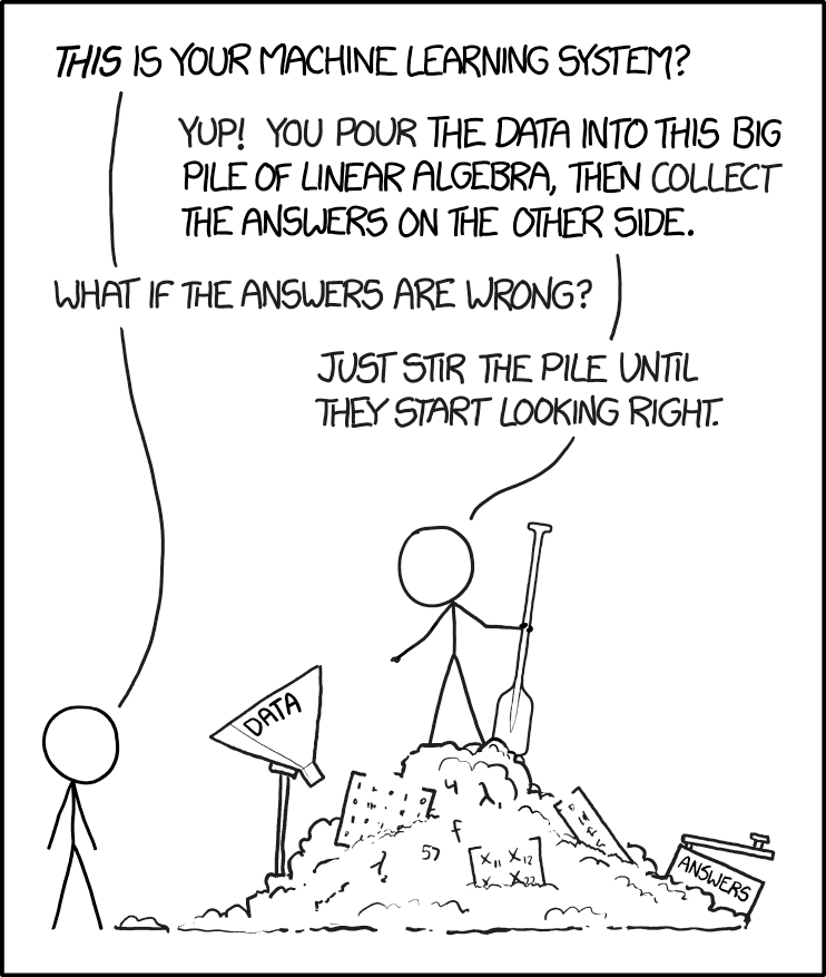
Figure 2. “Machine learning,” https://xkcd.com/1838/.
The parable presented in Figure 2 is about right: Without understanding the statistical foundations behind machine learning algorithms, you’re using tools without really knowing how they work (Lin et al 2025, more generally, see Downey 2024). We have a lot of work ahead of us, but, from time to time, we will exploit the power of AI and ML. For a start, I asked ChatGPT (August 2025), “What statistics is most relevant for ML?”, AI listed responses mapped to “Mike’s Biostatistics Book” are provided in Table 1.
Table 1. AI recommended core statistical topics matched to Mike’s Biostatistics Book
| ChatGPT recommended core statistics topics | Mike's Biostatistics Book |
|---|---|
| Descriptive statistics | Chapter 3 |
| Probability theory | Chapter 6 - 7 |
| Common probability distributions | Chapter 6 |
| Statistical inference | Chapter 8 |
| Estimation and Likelihood | Chapter 3, 6, 17 - 20 |
| Regression analysis | Chapter 17 - 18 |
| Analysis of Variance (ANOVA) | Chapter 12 - 14 |
| Resampling methods | Chapter 19 |
| Dimensionality reduction | Chapter 16, 20 |
| Time series and autocorrelation | Chapter 17 - 18, 20 |
| Optional: Bayesian statistics | Chapter 8 - 9, 18, 20 |
Biostatistics is embedded in bioinformatics and data science, in general. Thus, as implied by Figure 2, a critical step in working with datasets, whether small or large, is to ensure the inputs are valid. This holds across the dat science disciplines. Learning data processing tasks, data cleaning and, more generally, data wrangling are included in our biostatistics course.
Note 4: For larger data sets in the course we will introduce you to rattle, an R package that helps with data processing and data mining with access to simple hypothesis tests (eg, do groups differ?), and pattern detection (eg, correlations and dendrograms). For their required project, students in BI311 may elect to work with the R package targets to build automated data pipelines (eg, calculating growth rates for tomato germination experiments or the essential genes project in Genomics class (BI-308).
In what disciplines are biostatisticians employed?
.
One way to begin this discussion is to think about where statisticians work. The job market includes:
Health Science.
- Drug design, causes of diseases (many “causes” of cancers).
- Health Professional (nurses, physical therapists).
- Type of care and recovery period (importance of a person’s mood on health).
- Exercise regime and recovery from injury.
- Nutrition:- vitamins and health: diet and health.
Ecology & Evolution.
- Causes of changes in population sizes (conservation biology).
- Effects of pollution on organisms and ecosystems.
- Evolution of traits in populations over time.
- Global environmental changes and changes in population sizes or species diversity.
Genetics & Molecular Biology.
- Identifying genes that influence traits (eg, breast cancer, cystic fibrosis).
- Nature vs. nurture (heredity and environment effects on phenotypes).
- Multiple sequence alignment in comparative genomics.
Agriculture.
- Fertilizer effects on plant growth and productivity.
- Compare farming and harvesting methods (eg, organic vs conventional farming).
- Compare plant hybrids for differences in productivity.
Here’s a web site that keeps track of statistics jobs Biostatistics. I would go on to add that experience and competence in statistics would also translate to employment in non-biology fields, eg, business analytics.
Conclusions.
.
Moving forward, we have much to do — you will be exposed to many specific examples of statistical tests, how to calculate estimators, and how to make inferences from experiments. An important goal of this course is for you to be introduced and develop your ability to design experiments. why should you, as biologists and future health care providers, learn biostatistics?
- Develop statistical reasoning skills. Most, if not all graduate students will need to take several courses in statistics.
- Statements about research findings, new and better products, sociological and political issues often depend in large part on some form of statistical analysis.
- By learning a little about experimental design, sampling, and statistical testing, you will be much closer to being able to participate fully in these debates.
- Most, if not all graduate students will need to take several courses in statistics.
- Most, if not all jobs in biology require some training in statistics.
So, there’s really no doing biology without at least some knowledge of statistics. You’re getting a head start!
Questions
- Write up three learning outcomes for this page. Hint: Point your favorite generative AI to this page and ask for help.
- Explore current “biostatistics,” “bioinformatics,” and “data science” job prospects at Indeed.com or other recruiting sites. Search your area/city and also try a wider search.
- Given the rise of AI, now is a great time to explore current thinking about the future and need for biostatistics skills. Write a one paragraph perspective, your “worldview” about pros/cons of developing statistics and data science skill sets.
.
Quiz Chapter 2.1
Why (bio)statistics?
Chapter 2 contents
.
7.1 – Epidemiology definitions
Introduction
This subchapter may lack for drama, but let’s start by providing a list of key terms with definitions as you start our introduction to epidemiology. More definitions will follow in the sections as well.
Definitions
Absolute risk: The probability that a specified event will occur in a specified population. See Ch07.4 – Epidemiology: Relative risk and absolute risk, explained.
Absolute risk reduction (ARR): the decrease in risk of an event in an exposed (treatment) group compared to an unexposed (control) group. Also called the risk difference.  , see Contingency table. See Ch07.4 – Epidemiology: Relative risk and absolute risk, explained.
 : Control Event Rate and Experimental Event Rate. In observational studies, transition from “control” and “experimental” to exposure terms. For example, prospective or retrospective cohort studies,
 is Exposed Event Rate and its partner
 , Unexposed Event Rate. Equivalently, you will encounter
 for Incidence in the Exposed and
 forIncidence in the Unexposed. For Case-Control studies, where the direct event (incidence) rates over time are unavailable, then becomes Exposure Rate in Cases — the proportion of people with the condition who were exposed to the risk factor and
 is now Exposure Rate in Controls.
Contingency table, also called cross tabulation or crosstab, is a display of counts of variables in a matrix format. We briefly introduced the contingency table in Chapter 5.1. In epidemiology, rows of contingency table represent treatment or exposure groups, columns represent outcomes.
Table 1. A 2 X 2 contingency table
| Outcome | ||
| Yes | No | |
| Treatment or exposed group | a | b |
| Control or nonexposed group | c | d |
The 2X2 contingency table is referred to frequently in this chapter and again in Chapter 9.
R code
a = 4; b = 46; c = 5; d = 45

Table1 <- matrix(c(a,b,c,d), 2, 2, byrow=TRUE, dimnames = list(c("Treatment", "Control"), c("Yes", "No"))); Table1
R output
          Yes  No
Treatment   4  46
Control     5  45
In statistical classification, a field dedicated to establishing algorithms for correctly identifying and predicting classes of data, eg, correct disease diagnosis or , the 2X2 contingency table is often called a confusion or error matrix (Greene 2003). Machine learning methods are often built on developments from statistical classification findings (Michie et al 1995). We expand on contingency tables in Chapter 7.4 and Chapter 9.2.
Note 1: First discussed in Chapter 5.1, by convention, the standard format for an epidemiological 2×2 contingency table organizes exposure on the rows and disease outcome on the columns as follows:
- Rows (Exposure): The top row represents Exposed / Treatment (Yes), and the bottom row represents Non-exposed / Control (No).
- Columns (Outcome): The left column represents Disease / Case (Yes), and the right column represents No Disease / Control (No). See Chapter 7.
Control event rate (CER): How often an event occurs in the control group.  , see Contingency table.
Diagnosis: identification of the nature of a disease or condition.
Event: From probability theory, an event is a set of one or more outcomes to which a probability is assigned to each outcome.
Experimental event rate (EER): How often an event occurs in the treatment group.  , see Contingency table.
Exposure risk: the potential for harm from contact with or vulnerability to a hazard or risk factor.
Hazard: anything that can cause harm.
Incidence: the number of newly diagnosed individuals in a population having a condition, disease or other characteristic. Compare to prevalence.
Likelihood: In every-day English, the term likelihood and probability mean the same thing — the chance that an event will occur. In statistics, however, probability refers to possible outcomes in the future — a prediction for an event to occur, whereas likelihood is associated with the possible explanation (hypothesis) for the outcome that has already occurred, the past. Put another way, likelihood quantifies how likely is the data we observe, given the hypothesis (cf. excellent discussion by Gallistel 2015)? We will look at likelihood methods in practice in subsequent chapters.
Negative predictive value of a test (NPV), defined as the probability that a negative test result identifies a person who truly does not have the disease. Calculated as the total number of individuals without the disease divided by the total that tested negative. 
Number needed to treat (NNT): the inverse of the absolute risk reduction. 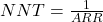 . See Ch07.4 – Epidemiology: Relative risk and absolute risk, explained.
Odds, the ratio (OR) of two probabilities: the probability of getting a one on throwing a dice is  , the probability of not getting a one is
 , therefore the odds of getting a one are 1 to 5.
 . See Ch07.5 – Odds ratio.
Outcome, the single result from a random experiment. For example, result of a single coin toss is “heads.” Results of a birth, the outcome is the child born is a singleton, single birth.
Per capita rate, Latin phrase, for each head, meaning per person.
Positive predictive value of a test (PPV), defined as the probability that a positive test result identifies a person who truly has the disease. Calculated as the total number of individuals with the disease divided by the total that tested positive. 
Posttest probability refers to the probability that the patient has the disease after the results of the test are known.
Pretest probability is the prevalence of the disease, ie, the chance that the a randomly selected person from the population has the disease.
Prevalence: The proportion of individuals in a population having a condition, disease, or characteristic. Compare to incidence.
Probability, defined in Chapter 6.1.
Prognosis, how a disease plays out.
Relative risk: Ratio of the risk of an event among those exposed to the risk factor to the risk among those not exposed to the risk factor. See Ch07.4 – Epidemiology: Relative risk and absolute risk, explained.
Relative risk reduction (RRR): is a measure calculated by dividing the absolute risk reduction by the control event rate. See Ch07.4 – Epidemiology: Relative risk and absolute risk, explained.
Risk: Probability of an event. Risk is not restricted to just bad events, but refers to the uncertainty of a particular event (eg, the risk that a child will be born male seems a melodramatic statement, but it is accurate as far as this definition goes).
Therapy, treatment intended to treat, relieve, or cure a disorder of condition.
Questions
- Compare and contrast ARR and RRR.
- What’s the difference between event, hazard, and risk?
- What’s the difference between incidence and prevalence?
- What’s the difference between diagnosis and prognosis?
- What’s the implication of a NNT greater than 100 in terms of the utility of a proposed therapy or treatment?
Quiz
Quiz Chapter 7.1
Epidemiology definitions
Chapter 7 contents
- Introduction
- Epidemiology definitions
- Epidemiology basics
- Conditional Probability and Evidence Based Medicine
- Epidemiology: Relative risk and absolute risk, explained
- Odds ratio
- Confidence intervals
- References and suggested readings
Preface
Overview.
.
The following pages, loosely called Mike’s Biostatistics Book, contain the extended versions of my lectures for BI311 Biostatistics, a biology course I teach at Chaminade University.
The companion site, Mike’s Workbook for Biostatistics, provides homework, problems and projects to learn-by-doing biostatistics, and several R tutorials. (I’ve also put together a number of handouts, background, and bioinformatics support at Mike’s Genetics & Genomics Workbook, consisting of materials used to support my lab classes these past 20 years.)
The Biology department faculty require biology majors to take this course. Class standing of students range from sophomores to first year graduate students.
We use and rely heavily on R, the open source “language and environment for statistical computing” (R-project [dot] org), and the R Commander package by J Fox (Fox 2005; Fox 2016). R Commander allows students to gain confidence with R commands by use of drop down menus to access functions. Increasingly, we also use Google CoLab to run simple R sessions.
The lecture notes are written from my perspective on what matters in a semester-long, first course in Biostatistics: concepts, context and practical advice along with a generous introduction to general linear models. The focus is on applied statistics with reference to other data science skill sets as needed. Concepts are illustrated by examples and multiple choice questions to “test” reader comprehension. Examples in Mike’s Biostatistics Book are generally from real data sets in biological or biomedical research. Therefore, context and practice comes from data sets we will work on throughout the semester. The data sets are presented in the accompanying workbook, body titled Mike’s Workbook for Biostatistics.
The material presented in Mike’s Biostatistics Book provide background and the examples needed to complete the problems presented in the course workbook.
- Chapter 2: Statistical reasoning.
- Workbook: Homework 1: Project data life cycle.
- Chapter 3 and 4: Exploring data.
- Workbook: Homework 2A: Descriptive statistics.
- Workbook: Homework 2B: Graphs.
- Chapter 5: Experimental design.
- Chapter 6: Probability.
- Workbook: Homework 3: Distributions & Probability.
- Chapter 7: Risk analysis.
- Workbook: Homework 4: Risk.
- Chapter 8: Inferential statistics.
- Workbook: Homework 5: Inference.
- Chapter 9: Qualitative (categorical) analyses.
- Workbook: Homework 6: Chi-square problems.
- Chapter 10 – 19: Quantitative (continuous) analyses.
- Chapter 10, 12, 13 – Workbook: Homework 7: t-tests and ANOVA.
- Workbook: Homework 8: Multiway ANOVA.
- Workbook: Homework 10: Correlation.
- Workbook: Homework 10: Multiple linear regression.
- Chapter 11: Power analysis.
- Chapter 15: Nonparametric tests.
- Chapter 19: Distribution-free methods.
- Chapter 20: Additional topics (partial listing).
- growth curves, dose response.
- logistic regression.
- others.
- Statistical tables.
- Appendix
While the intention is to downplay lists of statistical tests in favor of developing statistical reasoning, many of the kinds of tests one comes across are introduced and discussed in this book. The intent is to introduce these tests as special cases of general (or generalized) models from a data analyst’s point of view. Think of “k-means clustering“, “independent sample t-test“, “ANOVA“, “linear regression“, and the other tests as vocabulary. We understand biology best when we can talk the talk, and the same holds for learning statistics.
The book does not include machine learning — systems that can learn and help make decisions from data — and as of September 2023, includes only a short discourse on clustering and dimensionality reduction of data sets.
About this book (and website).
.
This textbook is an eBook and will undergo updates to correct errors, improve clarity, and even new content, throughout the semester. Although in spirit I welcome comments, corrections, and suggestions to improve coverage and content, I have closed comments at this site to minimize spam. As the book has a modest readership from multiple countries, I’m always happy to try and answer student questions — A little judicious search on the part of the reader likely will find a relevant email address.
Typesetting.
.
The manuscript was type set from a mix of html and Markup language — See Part 09: Making a report at Mike’s Biostatistics Book — and Ghostwriter (version 2 [dot] 1 [dot] 1), and the eBook (pdf version coming soon!) was generated and edited with Calibre (version 5 [dot] 35 [dot] 0).
Text to speech considerations.
Text to speech apps can get confused when a period appears within text and not just at the end of a sentence. Therefore, I’ve dropped periods from “Fig. 1” and the “e.g.” and “i.e.” Latin abbreviations. Periods appear in R commands, for example, data.frame(), and those remain as is. Similarly, I generally add a period after a subheading to encourage a break by text to speech apps.
Hosting.
Both books, Mike’s Biostatistics Book and Mike’s Workbook for Biostatistics, are hosted on my website. This site, Mike’s Biostatistics Book, is solely supported by me and I don’t monetize the site. As of Fall 2023, the site cookie only stores temporary session information during a users visit.
Equations.
.
Equations in the eBook were created with LaTeX — a software system used to prepare and format documents — and saved as PNG images, or embedded in text (QuickLaTeX WordPress plug-in). Pages with many images or equations may be slow to load in your browser: in general, to improve browsing experience reduce the number of open tabs and use of additional apps.
References and citations.
.
Introductory textbooks often lack in-line citations. The absence of in-line citations improves readability, but at the very real expense of giving credit to the original and to providing the reader the opportunity to verify facts and opinions presented. I have tried a balance: first, I included in-line citations to references. One of many remaining tasks for me to improve the book is to complete linkage of in-page citations to reference lists. I have, however, refrained from an exhaustive, dissertation-like reference listing for each point raised in the book. Second, most citations are to open access articles (or articles with pdfs available by judicious search), with the justification of the reader has access to the original material. However, this approach is a form of citation bias. Thus, I refer to reference pages as References and Suggested Readings, and don’t claim Mike’s Biostatistics Book as an authoritative voice on the subject (cf. discussion in Greenberg 2009 Bmj 339).
A note about me.
.
I’m an Associate Professor of Biology at Chaminade University. My PhD was not in statistics, I trained in evolutionary physiology and quantitative genetics. Quantitative genetics is an applied field that depends heavily on use of mathematics and statistics, particularly linear models. I took courses in applied statistics while at the University of Wisconsin, but I would not call my training in statistics thorough or complete. Much of what I know comes from self-study. My strengths in biostatistics, I believe, are in translation of sometimes dense mathematics to direct use and application. Thus, I have developed a direct style to the material that I hope you will find helpful as you work on the material. It also means we won’t spend a lot of time with proofs, not because these are unimportant, but because they can side-track from developing your statistical thinking when it comes to data analysis — but primarily because this is not my strength. References are presented in the book to support the algorithms and mathematical foundations of biostatistics and to back claims I make about applied statistics.
Thus, I don’t claim that I have all of the answers, nor am I saying that the mathematical foundations are unimportant, far from it. But we have to start somewhere and I elect to spend our time on the concepts in statistics, the why do we do it this way, as opposed to the mechanics of the mathematics, the how do we do it.
What I have learned about statistics comes from publications from many real statisticians; Mike’s Biostatistics Book, such as it is, stands on on their work. I apologize in advance to any author whose work has not been given proper credit. Mistakes or mischaracterizations are, of course, mine alone.
Other sources of expertise.
.
Mike’s Biostatistics Book of lecture notes is intended to provide students with a foundation in biostatistics: the concepts of assumptions, probability, sampling, description, and modeling that support a researcher’s ability to advance knowledge in biology. But you will very much benefit from other opinions, other voices. And, as much as I have adopted the online presence, it is hard to beat a book in hand as a guide. Good statistics books retain their value well passed their publication date. Some of the textbooks I have found useful over the years include the following:
Introduction and general statistics.
.
Chaterjee S, Price B (1977) Regression analysis by example. Wiley Interscience (5th edition now published in 2006)
Glover T, Mitchell K (2008) Introduction to biostatistics, 2nd edition. Waveland Press
Norman GR, Streiner DL (2003) PDQ Statistics, 3rd edition. BC Decker
Snedecor GW, Cochran WG (1989) Statistical methods, 8th edition. Iowa State University Press
Sokal RR, Rohlf (1981) Biometry, 2nd edition. WH Freeman (4th edition published in 2011)
Whitlock MC, Schluter D (2008) The analysis of biological data. Roberts and Company
Zar J (1999) Biostatistical analysis, 4th edition. Prentice Hall (5th edition published in 2011)
Intermediate and advanced books.
Abelson RP (1995) Statistics as principled argument. Taylor & Francis (epub available)
Bulmer MG (1967) Principles of statistics. Dover Publications (epub available)
Davidson AC, Hinkley DV (1997) Bootstrap methods and their application. Cambridge University Press (epub available)
Edwards AWF (1992) Likelihood, expanded edition. Johns Hopkins University Press
Fisher RA (1934) Statistical methods for research workers, 5th edition. Oliver and Boyd (The last edition was the 14th)
Härdle W, Simar L (2003) Applied multivariate statistical analysis. Springer-Verlag
Lee PM (1989) Bayesian statistics: An introduction. Oxford University Press – McCullagh P, Nelder JA (1989) Generalized linear models, 2nd edition. Chapman and Hall
Montgomery DC, Peck EA (1992) Introduction to linear regression analysis, 2nd edition. John Wiley & Sons (5th edition published in 2013)
Neter J, Wasserman W, Kutner MH (1989) Applied linear regression models, 2nd edition. Robert D Irwin (4th edition published in 2003)
Quinn GP, Keough MJ (2002) Experimental design and data analysis for biologists. Cambridge University Press.
Shao J (2003) Mathematical statistics, 2nd ed. Springer Science
Wei WWS (1990) Time series analysis. Addison-Wesley (2nd edition published in 2005)
Some of these titles are old!
.
One of the good things about statistics is that many of the standard statistical applications were developed a long time ago, so “old textbooks” in statistics retain their value. A quick search online will result in many options to purchase one or more of these books for under $10. In addition, most of the books listed above have new editions; where appropriate I have listed the most recent available edition.
What about books on R?
None of the listed books teach R. Between Mike’s Biostatistics Book and the companion Mike’s Workbook for Biostatistics, several tutorial and lots of worked examples are provided to help you learn how to use R to help statistical work. A quick Google search, e.g., “free online books learn R,” returns thousands of suggested titles. Search “R tutorials,” for millions more. Chances are, if you have a question about how to do some task in R, someone has already solved the task and published code examples for you to borrow (always cite your sources!).
Concluding remarks about these lecture notes.
.
These collected lecture notes will serve as your official textbook – I have tried to make them accurate, informative, and yet balanced between providing too much detail while still providing depth to the presentation. In class, lecture slides will be provided as outline to these more extensive notes. Homework and quizzes support the progress through the notes.
The lecture notes contained in Mike’s Biostatistics Book are very much a work in progress, with some areas more developed than others. If you find areas that make no sense, seem abrupt, or you would like more examples, please do let me know. Your input is important to improve this textbook; the Discussion Forum on the course website is a good place to do lend your critiques and suggestions.
Like most subjects one voice is not enough; you will benefit from acquiring a second opinion, either from one or more of the books listed above or from the many online sites on statistics you will find. The good news is that you will find substantial overlap between what I write and other sources you may acquire because the topics we will cover are foundational and my take is mainstream.
However, you will also find some differences in detail. For one example, I have included much more on risk analysis and an epidemiology tilt as compared to many of the the titles listed under the Introduction and General statistics category. For a second example, I give a different perspective on how to work with probability calculations, emphasizing use of natural numbers over frequency calculations. Many examples provided in the book are drawn from data sets created in lab classes or as preliminary and pilot projects from my research at Chaminade University: growth curves, dose-response, working with RT-PCR traces, multi-well plate assays and more.
Preface contents
.
Preface