6.2 – Ratios and probabilities
Introduction
One common objective of a research project is comparison between quantities: one effective way to communicate a comparison is to construct a ratio. Ratios provide a standardized way to compare different data sets. The purpose of this page is introduce the wealth of types of ratios used for quantification of comparisons, from indexes to ratios.
Let’s review our definitions again. An event is some occurrence. As you know, a ratio is one number, the numerator, divided by another called the denominator. A proportion is a ratio where the numerator is a part of the whole. A rate is a ratio of the frequency of an event during a certain period of time. A rate may or may not be a proportion, and a ratio need not be a proportion, but proportions and rates are all kinds of ratios. If we combine ratios, proportions, and/or rates, we construct an index.
Ratios
Yes, data analysis can be complicated, but we start with this basic idea. Much of the statistics is based on frequency measures, eg, ratios, rates, proportions, indexes, and scales.
Ratios are the association between two numbers, one random variable divided by another. Ratios are used as descriptors and the numerator and denominator do not need to be of the same kind. Business and economics are full of ratios. For example, return on investment (ROI), eg, earnings equals net income divided by number of shares outstanding, the Price-Earnings, or P/E ratio, is the ratio of the price of a stock to the earnings per stock, as well as many others are used to summarize performance of a business, and to compare performance of one business against another.
Note 1: ROI also stands for region of interest — a sample in a data set identified by the analyst for a particular interest. Often refers to a specific area in an image.
Ratios are deceptively convenient way to standardize a variable for comparisons, ie, how many times one number contains another. For example, when estimating bird counts for different areas, or different birding effort (intensity, time searched), we may correct counts by accounting for area in which counts were made or the total time spent counting, for a per-unit ratio (Liermann et al 2004).
Practice: There were 1,326 day undergraduate students enrolled in 2014 at Chaminade University of Honolulu and the Sullivan Library added 8469 new items (ebooks, journals, etc,) to its collection during 2014. What is the ratio of new items per student?

Data collected from Chaminade University website at www.chaminade.edu on 3 July 2014.
Practice: For another example, what is ratio of annual institutional aid a student at Chaminade University may expect to receive compared to a student at Hawaii Pacific University?

Thus, in 2014, Chaminade offered more than twice the institutional aid to its students then does HPU (both institutions are private universities, data from retrieved on 3 July 2014 from www.cappex.com).
Relative change, Fold-change and orders of magnitude
It’s common practice to report on the amount of change between two quantities recorded over time. Relative change (often percentage) describes change relative to an initial value. Relative change in root length b
To make percent increase (decrease), simply multiple 100%.
(1) 
The ratio between two quantities, eg, to compare mRNA expression levels of genes from organisms exposed to different conditions, researchers may report fold-change. Fold change is often reported as log base 2 change.

Why log base 2? Symmetry and ease of reporting. A doubling becomes +1 and a halving becomes -1. Without log transformation, doubling is +2, but having is +0.5.
Relative change is useful for reporting percent changes, fold change for ratios, although if the change is small in amount, then relative change can be misleading, eg, value goes from five to ten, then the relative change is 100%, but effectively, a very small change in absolute units. Similarly, fold change becomes a large, but likely meaningless comparison, if the denominator is close to zero.
An example of calculation of fold change. Rates of the expression from cells exposed to heavy metal divided by expression under basal conditions. Gene expression under different treatments may be evaluated by calculating fold-change as the log base2 of the ratio of expression of a gene for one treatment divided by expression of same gene from control conditions. Copper is an essential trace element, but excess exposure to copper is known to damage human health, including chronic obstructive pulmonary disease. One proposed mechanism is that cell injury promotes an epithelial-to-mesenchymal shift. In a pilot study (N.I.H. INBRE P20RR016467), we investigated gene expression changes by quantitative real-time polymerase chain reaction (qPCR) in a rat lung Type II alveolar cell line exposed to copper sulfate compared to unexposed cells. Record cycle threshold values, CT, for each gene, where CT is number of cycles required for the fluorescent signal to exceed background levels; CT is inversely proportional to amount of cDNA (mRNA) in the sample. Genes investigated were ECAD, FOXC2, NCAD, SMAD, SNAI1, TWIST, and VIM, with ATCB as reference gene. ECAD expression is marker of epithelial cells, whereas FOXC2, NCAD, SNAI1, TWIST, and VIM expression marker of mesenchymal cells. After calculating  values, geometric means of normalized values of three replicates each are shown in Table 1.
Note 2: The  is a relative change quantification that relates the PCR signal of the normalized gene of interest (GOI) transcript in a treatment group to another sample, eg, an untreated control. is now a widely applied method to analyze the relative changes in gene expression from real-time quantitative PCR experiments (relevant papers on the analysis method, Livak and Schmittgen (2001) and Schmittgen and Livak (2008) have been cited more than 230K times, Pubmed 2026. See also Rao et al (2013).)
Log-transform, introduced in Ch03.2, was used because gene expression levels vary widely on the original scale and any log-transform will reduce the variability. log-base 2 specifically was used for fold-change in particular because it is easy to interpret (eg, see discussion in Bergemann and Wilson 2011 and Corliss et al 2024), and provides symmetry (all log-transforms provide this symmetry). For example, log(1/2, 2) returns -1, while log(2/1, 2) returns +1. Thus, base 2, we see a decrease by half or doubling of original scale is a fold change of  . In contrast,
log(1/2, 10) returns -0.301, while log(2/1, 10) returns +0.301 — which is perfectly accurate, but deceptive to interpret.
log-base 2 is commonly employed to calculate the number of bits — binary digits — for a given number of values. For example, 8 bits (0 – 7), then log2(8-1), and R returns 2.807355. Round, add 1, and the number of bits is3. Related R code, if want to calculate and print te binary representation of of a number, eg, 8, try
myBits <- intToBits(8)
paste(as.character(myBits),collapse="")
On a more casual note, log-base 2 is useful to calculate number of rounds for a single-elimination playoff tournament, eg, NCAA men’s and women’s basketball tournament or March Madness (NCAA). As of 2025, 60 teams are invited, plus the four winning teams from four play-in games, for a total of 64 teams. The number of rounds is log2(64) and R returns 6. These six are referred to as First Round, Second Round, Sweet Sixteen, Elite Eight, Final Four, and the Championship Game. The play-in games are referred to as the”First Four.” The function draw_bracket() of R package SwimmeR can be used to plot a simple playoff bracket.
Table 1. Mean and fold change of gene expression values from qPCR for several genes from a rat lung cell line.*
| Control | Copper-sulfate | Fold change | |
| ECAD | 34.6 | 35.7 | 0.6 |
| NCAD | 28.5 | 24.0 | 27.2 |
| SMAD | 29.5 | 25.0 | 28.2 |
| SNAI1 | 25.5 | 28.1 | 0.2 |
| FOXC2 | 27.6 | 27.0 | 1.9 |
| VIM | 23.1 | 16.4 | 134.4 |
| TWIST | 25.1 | 22.9 | 5.6 |
* INBRE funding, P20RR016467.
At face value, following four hour exposure to copper sulfate in media, some evidence that the epithelial cell line adopted gene expression profile of mesenchyme-like cells. However, weakness of fold-change is clear from Table 1: the quantity is sensitive to small values. ECAD expression in the cell line is low, thus high numbers of PCR cycles (mean = 36) and treated cells not much fewer (mean = 34.4).
Note 3: Calculation of is included. Geomean CT were
| Control | CuSO4 | |
| ACTB | 32.2 | 32.5 |
| NCAD | 28.5 | 24.0 |
For control cells, 
For treatment cells, 
and 
log2, 
table value differs by rounding
Orders of magnitude
In addition to fold change, order of magnitude is another common way to compare quantities. While fold change returns the multiplier between two numbers, order of magnitude generally refers to differences in multiples of ten, logarithmic.

Thus, a difference of one order of magnitude is the number multiplied by 101, three orders of magnitude is the number multiplied by 103, and so on. A change from 10 to 100 is a one order of magnitude increase; the same change, 10 to 100, is a ten-fold change. It’s a difference of scale. If a person’s salary increases by 3%, from $49K to $50,470, reporting this as an “order of magnitude” increase is nonsensical as a communication device (magnitude of change is just 0.01). By contrast, fold change for the same increase would be 1.03 — also indicative of a negligible increase, but a cleaner representation.
Rates
Rates are a class of ratios in which the denominator is some measure of time. For example, the four year graduation rate of some Hawaii universities are shown in Table 2.
Table 2. Percent students graduation with bachelor’s degrees within four years or six years (cohort 2014, data source NCES.ed.gov)
| School | Private/Public | Four-year, Percent graduation |
Six-year, Percent graduation |
| Chaminade University | Private (non-profit) | 43 | 58 |
| Hawaii Pacific University | Private (non-profit) | 31 | 46 |
| University of Hawaii – Hilo | Public | 15 | 38 |
| University of Hawaii – Manoa | Public | 35 | 62 |
| University of Hawaii – West Oahu | Public | 16 | 39 |
| University of Phoenix | Private (for profit) | 0 | 19 |
Examples of rates
Rates are common in biology. To name just a few
- Basal metabolic rate (BMR), often measured by indirect calorimetry, reported in units kiloJoules per hour.
- Birth rates and mortality (death) rates, components of population growth rate.
- Extinction rate, how often over a given time species go extinct.
- Growth rate, which may refer to growth of the individual (somatic growth rate), or increase of number of individuals in a population per unit time.
- Molecular clock hypothesis, rate of amino acid (protein) or nucleotide (DNA) substitution is approximately constant per year over evolutionary time.
- Mutation rate, frequency of new mutations in a DNA sequence of an organism over time.
- Photosynthetic rate, convert light energy into chemical energy.
- Phred quality score, error rates of incorrectly called nucleotide bases by the sequencer.
Proportions
Proportions are also ratios, but they are used to describe one part to the whole. For example, 902 women (self-reported) day undergraduate students enrolled in 2014 at Chaminade University in Honolulu, Hawaii.
Practice: Given that the total enrollment for Chaminade in 2014 was of 1,326, calculate the proportion of female students to the total student body.

More practice: A common statistic in agriculture is germination percentage, count the number of seeds that sprout over a period of time divided by total number of seeds planted multiplied by 100. Figure 1 shows an example of a germination trial for five tomato seeds. Seed in position 3 (left to right 1 – 5) failed to germinate, whereas the other four seeds display range of seedling growth. (A seed coat is observed next to plant 2.)

Figure 1. Example planting of five tomato seeds, day 5, on agar Petri dish (M. Dohm).
Observations conducted over 10 days. Germination defined as evidence of radicle by day 10. Data collected by student for biostatistics project. A random sample of results from three plates is presented in Table 3.
Table 3. Germination of tomato seeds on agar Petri dishes.
| Plate* | 1 | 2 | 3 | 4 | 5 |
| 18 | Yes | No | Yes | Yes | Yes |
| 13 | Yes | Yes | Yes | No | Yes |
| 20 | No | Yes | Yes | Yes | Yes |
* Random sample of three plates drawn from among 30 plates.
We calculate the percent germination for the 15 seeds planted as

Thus, for the sample of plates the germination percent was 80%, which, coincidently, is the same result if germination percent was calculated for the five seeds displayed in Figure 1.
Beginning in Chapter 7 – Probability, Risk Analysis, we introduce and use a number of proportions, for example incidence and prevalence are proportions, as is PPV — positive predictive value. Sensitivity and specificity are both proportions and also qualified as indexes.
Comparing proportions
In some cases you may wish to compare two proportions or two ratios. The hypothesis tested is the difference between the two ratios, and the test is if the confidence interval of the difference includes zero. If it does, then we would conclude there is no statistical difference between the two proportions. In R, use the prop.test function. For example, 63 women were on team sport rosters at Chaminade in 2014, a proportion of 59% of all student athletes (n = 106). Recall from the example above that women were 68% of all students at Chaminade University. Title IX compliance requires that a university “maintain policies, practices and programs that do not discriminate against anyone on the basis of gender” (NCAA, INCLUSION AND BELONGING Championing Women in Sports). In terms of athletic programs, then, universities are required to provide participation opportunities for women and men that are substantially proportionate to their respective rates of enrollment of full-time undergraduate students.
Consider Chaminade University: Is there a statistical difference between proportion of women athletes and their proportion of total enrollment? We introduce statistical inference in Chapter 8, but for now, this is a test of the null hypothesis that the difference between the two proportions is zero.
At the R prompt type (remember, anything after the # sign is a comment and ignored by R).
women = c(62,902)  #where 62 is the number of women athletes and 902 is the number of women students
students = c(106,1326)  #106 is the number of student athletes and 1326 is all students
prop.test(women,students)  #the default is a two-tailed test, ie, no group differences
And R returns
2-sample test for equality of proportions with continuity correction
 data: women out of students
X-squared = 3.6331, df = 1, p-value = 0.05664
alternative hypothesis: two.sided
95 percent confidence interval:
 -0.197532407 0.006861073
sample estimates:
 prop 1 prop 2
0.5849057 0.6802413
What is the conclusion of the test?
When you compare two groups, you’re asking whether the two groups are equal (the null hypothesis). Mathematically, that’s the same as saying the difference between the two groups is equal to zero.
First check the lower and upper limits of the confidence interval. A confidence interval is one way to report a range of plausible values for an estimate (see Ch 7.6 – Confidence intervals). It’s called a confidence interval because a probability is assigned to the range of values; a 95% confidence interval is interpreted as we’re 95% certain the true population value is somewhere between the reported limits. For our Chaminade University Title IX question, recall that we are asking whether the value of zero is included. The lower limit was -0.1975 and some change; the upper limit was 0.0068 and some change. Thus, zero is included and we would conclude that there was no statistical difference between the two proportions.
The second relevant output to look at is the p-value, or probability value. If the p-value is less than 5%, we typically reject the tested hypothesis. We will talk more about p-values and their relationship to inference testing in Chapter 8; for now, pay attention to the confidence interval (introduced in Chapter 3.4); if zero is included, then we conclude no substantial differences between the two proportions.
Indexes
Indexes are composite statistics that combine indicators. They condense complex diagnostic performance data into a single, universally understood numerical indicator.
Indexes are common in biology, and well-known business and economics indexes are reported on every day, eg, Dow Jones Industrial average combines stock prices from 30 companies listed on the New York Stock Exchange and the CPI, or Consumer Protection Index, constructed by the US Bureau of Labor Statistics from a “market basket of consumer goods and services, used by the government and other institutions to track inflation. The CPI itself is made up of numerous indexes to account for regional price differences and other factors.
Some indexes presented in this book include
- Grade point average
- Body Mass Index (BMI)
- Comet assay indexes (tail intensity, tail length, tail moment) are used to assess DNA damage among organisms exposed to environmental contaminants (eg, Mincarelli et al., 2019).
- Encephalization index, ratio of brain to body weight among species. Used to compare cognitive abilities.
- Sensitivity, specificity, NNT — number needed to treat, odds-ratio and RRR and related. See Chapter 7.1 – Probability, Risk Analysis.
- Species diversity indexes, measures of species richness and abundance. See Chapter 20.8.
Scales
Agreement scales for surveys, eg, Likert scale or sliding scale (Sullivan and Artino 2013). For example, after learning about Theranos, students were asked:
How serious is this violation in your opinion?
| Not serious
0 |
Slightly serious
0 |
Moderately serious
2 |
Serious
4 |
Very serious
19 |
a 5-point scale.
Although an intuitive measure, how fast can an individual run, challenging to determine whether individual’s performance is at physiological maximum. Particularly for measures of performance capacity that involves behavior (motivation), may apply a race quality scale (eg., binary scale “good” or “bad” Husak et al 2006).
These examples reflect ordinal scales. Many of the nonparametric tests discussed in Chapter 15 are suitable for analysis of scales.
Limitations of ratios
Although the indexes may be easy to communicate, statistically, indexes have many drawbacks. Chief among these, variation in ratios may be due to change in numerator or denominator. Ratios and any index calculated by combining ratios seem simple enough, but have complicated statistical properties. Over the years, several authors have made critical suggestions for use of ratios and indexes. Some key references are Packard and Boardman (1988), Jasienski and Oikos (1999), Nee et al (2005), and Karp et al (2012). For example, ratios, computing trait value by body weight, are often used to compare some trait among individuals or species that differ in body size. However, this normalization attempt only removes the covariation between size and the trait if there is a 1:1 relationship between size and the trait. More typically, relationship between the trait and body size is allometric, ie, the slope is not equal to one. Thus, ratio will over-correct for large size and under-correct for small size. The proper solution is to conduct the comparison as part of an analysis of covariance (ANCOVA, see Chapter 17.6).
Example
Which is the safer mode of travel: car or airplane?
The following discussion covers travel safety in the United States of America for a typical year, 2000*.
Note 4: *The following discussion excludes the 241 airline passenger deaths associated to the terrorist attacks of September 11 2001 in the USA; the NTSB also “…exclude(s illegal acts) for the purpose of accident rate computation. It also does not include considerations of 2020-2021 and effects of the COVID-19 pandemic on numbers of flights. The purpose of this discussion is not to convince you about the safety of modes of travel. Moreover, the following analysis is not necessarily the proper way to frame or analyze risk, but, rather, the purpose of this discussion is to highlight the impact of assumptions on estimating risk.
Between 2000 and 2023, there were 779 deaths associated with accidents of major air carriers in the USA. Year 2009 was the last multiple-casualty crash of a major U.S. carrier (Colgan Air Flight 3407); between 2010 and 2021, two fatal accidents, two fatalities were reported.
We’ve all heard the claim that it’s much safer to fly with a major airline than it is to travel by car (eg, Flying is getting scary. But is it still safe? CNN June 20, 2024). There are a variety of arguments, but one statistical argument goes as follows. In 2000 in the United States, 638,902,993 persons traveled by major air carrier, whereas there were 190,625,023 licensed drivers. In 2000, 92 persons died in air travel (again, major carriers only), whereas 37,526 persons died in vehicle crashes (includes drivers and passengers). Thus, the risk of dying in air travel is given as the proportion  , or 1.44e-07 (0.000014%), whereas the comparable proportion for death by motor vehicle is
 , or 1.97e-04 (0.0197%).
In other words, we can expect one death (actually 1.4) for every ten million airline passengers, but 20 deaths (actually 19.7) for every one hundred thousand licensed drivers. Thus, flying is a thousand times safer than driving (actual result 1,367 times; divide the rate of motor vehicle-caused deaths for licensed drivers by the rate for airlines). Proportions are hard to compare sometimes, especially when the per capita numbers differ (ten million vs. 100,000 in this case).
We can put the numbers onto a probability tree and get a sense of what we are looking at (Fig 2).
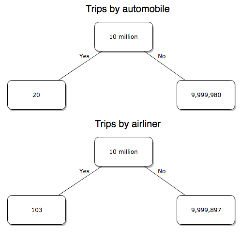
Figure 2. A probability tree to help visualize comparison of deaths (“yes”) by car travel and by airline travel in the United States for the year 2000.
Comparing rates and proportions
Without going into the details, we will do so in Chapter 9 Inferences on Categorical Data, comparing two rates is a chi-square, χ2, contingency table type of problem. More specifically, however, it is a binomial problem (Chapter 3.1, Chapter 6.5); there are two outcomes, death or no death, and we can describe how likely the event is to occur as a proportion. Because the numbers are large, we can use rely on the normal distribution for comparing the two proportions. We’ll explain this more in the next chapters, but for now it may be enough to present the equation for the comparison of two proportions under the assumption of normality, proportion z test.
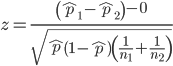
and the null hypothesis (see Chapter 8) tested as that the two proportions are equal. This may be written as
H0 : p1-p2=0
We can assign statistical significance to the differences in events for the two modes of travel under this set of assumptions. Rcmdr has a nice menu-driven system for comparing proportions, but for now I will simply list the R commands.
At the R prompt type each line then submit the command.
total = 100000000
prop.test(c(19700,14),c(total,total)))
And the R output
prop.test(c(19700,14),c(total,total))

    2-sample test for equality of proportions with continuity
    correction

data:  c(19700, 14) out of c(total, total)
X-squared = 19658, df = 1, p-value < 2.2e-16
alternative hypothesis: two.sided
95 percent confidence interval:
 0.0001940984 0.0001996216
sample estimates:
  prop 1   prop 2
1.97e-04 1.40e-07
There’s a bit to unpack here. R is consistent; when it reports results of a statistical test, it typically returns the value of the test statistic (χ2 = 19658), the degrees of freedom for the test (df = 1), and the p-value (< 2.2e-16).
prop.test() were calculated by the Wilson Score method not the Wald method. While both are parametric tests and therefore sensitive to departures from normality (see Chapter 13.3), formulation of Wilson score method makes fewer assumptions (involving approximations of the population proportions) and therefore is considered more accurate.By convention in statistics, if a p-value, where “p” stands for probability, is less than 5%, we would say that our results are statistically significant from the null hypothesis. Looks pretty convincing to me, the difference of 19,700 deaths compared to 14 deaths is clearly different by any criterion and by the results of the statistical test, the p-value is several orders of magnitude smaller than 5%.
Safer to fly. By far, not even close. And similar conclusions would be reached if we compare different years, or averages over many years, or if we used a different way to express the amount of travel (eg, miles/year) by these modes of transportation.
Are you convinced, really? Is it safer to fly?
Let’s try a little statistical reasoning — what assumptions did I make to do these calculations? We recognize immediately that many more people travel by car: that there are way more cars being driven then there are airline planes being flown. The question then is, have we properly adjusted for this difference? Here are a few considerations. My source for the numbers is the NTS 2001 book published by the U.S. Department of Transportation (U.S. Department of Transportation). We are conducting a risk analysis, and the first step is to make sure that we are comparing “apples with apples.” Here are two alternative solutions that at least compare, “Red Delicious” apples with “Macintosh” apples.
Option 1. There are many, many more licensed drivers than there are licensed commercial airline pilots. The standard comparison offered in the background above compared deaths per licensed car driver, but a different metric for air travel, the rate per passenger. This isn’t as bad of a comparison as it may seem — after all, the majority of deaths in car accidents are of the driver themselves. But it isn’t that hard to make the direct comparison — just find out how many commercial pilots there are — a direct comparison with licensed car drivers (stated above as 190,625,023). From the FAA we see that in 2009 there were 125,738 persons with commercial certificates. Since there are only 20 major airline carriers in the United States now (a few more were active in 2000, but we’ll put this aside), the number of licenses is an over estimate of the actual number we want — how many pilots of commercial airlines — but lets use this number for starters — after all, just because a person has a drivers license doesn’t mean they drive or ride in a car.
Number of deaths/yr: Let’s use 2000 data, a typical year prior to 9/11 (and excluding the Covid-19 pandemic). Airlines: 92 deaths; motor vehicles (includes passenger cars, trucks, etc, but not motorcycles): 37,526 deaths (drivers = 25,567; passengers = 10,695; 86 others).
Which mode of travel is riskier? I get a rate a rate of 7.3 X 10⁻⁴ deaths per commercial pilot, or
92125738
compared to a rate for car drivers of 1.97 X 10⁻⁴ deaths.
To summarize what we have so far, I get a result that suggests car travel is almost four times safer
7.3 x 10-41.97 x 10-4→7.31.97 = 3.7
then traveling by commercial airliner. In whole numbers, these results translate to seven deaths for every 10,000 commercial pilots compared to two deaths for every 10,000 licensed car drivers (Fig 3).
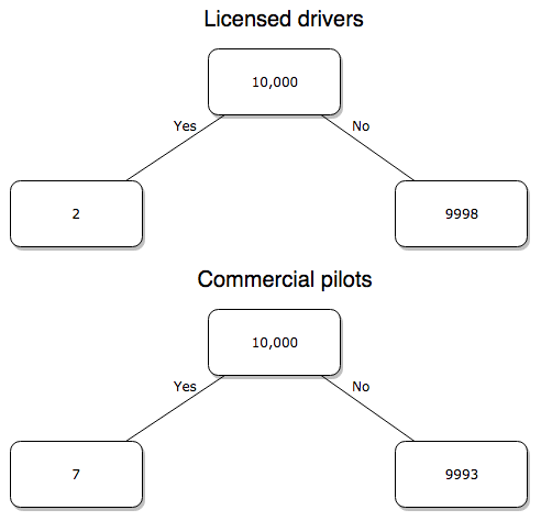
Figure 3. Comparing totals of deaths adjusted by numbers of licensed drivers and by licensed commercial airline pilots in the United States.
R work follows. Enter and submit each command on a separate line in the script window
total = 10000
prop.test(c(2,7),c(total,total))
And the R output
prop.test(c(2,7),c(total,total))

    2-sample test for equality of proportions with continuity
    correction

data:  c(2, 7) out of c(total, total)
X-squared = 1.7786, df = 1, p-value = 0.1823
alternative hypothesis: two.sided
95 percent confidence interval:
 -0.001187816  0.000187816
sample estimates:
prop 1 prop 2
 2e-04  7e-04
What’s happened? The p-value (0.1823) is not less than 5% and so we would conclude under this scenario that there is no difference between the proportions of deaths between the two modes of travel. Let’s keep going.
Option 2. There are many, many more cars on the road then there are airplanes flying commercial passengers. The standard comparison offered in the background information above identified death rates per individual driver, but used a different metric for airline travelers (number of deaths per passenger), which confuses individuals with travelers: what we need is the number of individuals that traveled by airliner, not the total number of passengers (which is many times higher, because of repeat flyers). How can we make a fair comparison for the two modes of travel? Most people never fly whereas most people drive (or ride in a car) frequently in the United States. To me, risk of travel might be better expressed in terms of a per trip rate. I want to know, what are my chances of dying each time I get into my car versus each time I fly on a commercial jet in the United States?
Number of trips/yr. For airlines, I use the number of departures (2000 = 8,951,773). But for cars, we need to decide how to get a similar number. It’s not available directly from the DOT (and would be difficult to get — studies with randomly selected drivers can yield as many as 5 trips per day for licensed drivers). I took the number of licensed drivers and bound the problem — at the low end, let’s say that only 2 trips per week (eg, 50 weeks) are taken by licensed drivers (100 trips); at the upper end, let’s take 2 trips per day per week, or 500 trips/year. Thus, at the low end, we have 1.91 X10¹⁰ trips per year; at the upper end, 9.53 X 10¹⁰ trips per year.
Which mode of travel is riskier? Using the number of deaths/yr listed above in Option 1, I get a rate of 1.03 X 10⁻⁵ deaths/trip for air carriers
928.95 x 10⁶
compared to a rate of 1.97 X 10⁻⁶ deaths/trip for cars (lower bound) or 3.9 X 10⁻⁷ deaths/trip for cars (upper bound). Here’s what the numbers look for in a tree (taking the lower number of trips per year for cars, Fig 4).
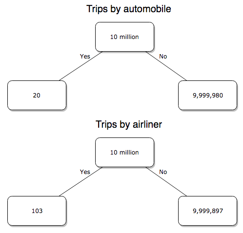
Figure 4. Comparing totals of deaths adjusted by numbers of car trips and by numbers of airline trips in the United States.
R work follow
total = 10000000
prop.test(c(20,103),c(total,total))
And the R output
prop.test(c(20,103),c(total,total))

    2-sample test for equality of proportions with continuity
    correction

data:  c(20, 103) out of c(total, total)
X-squared = 54.667, df = 1, p-value = 1.428e-13
alternative hypothesis: two.sided
95 percent confidence interval:
 -1.057370e-05 -6.026305e-06
sample estimates:
  prop 1   prop 2
2.00e-06 1.03e-05
Now we have another really small p-value (1.428e-13), which suggests a statistically significant difference between the modes of air travel, but the difference in deaths is switched. I now have a result that suggests car travel is much safer than traveling with a commercial airliner! These calculations suggest that you are as much as 26 (upper bounds, five times for lower bounds) times more likely to die from a plane crash then you are behind the wheel. In whole numbers, these results indicate one death for every 100,000 airline flights compared to 1 death for every 500,000 (lower estimate) or 2,500,000 car trips!
Do I have it right and the standard answer is wrong? As Lee Corso used to say on ESPN’s College GameDay program, “Not so fast, my friend!” (Wikipedia). Mark Twain was right to hold the skeptic’s view. Begin by listing the assumptions and by checking the logic of the comparisons (there are still holes in my logic!!). For one, if I am considering my risk of dying by mode of travel, it is far more likely that I will be in a car accident than I will an airline accident, simply because I don’t travel by airline that much. When we consider lifetime risk, we can see why the assertion that it is “safer to fly than drive” is true — we’re far more likely to belong to one of the reference populations involving automobiles (eg, those who drive frequently, for many years) than we are to be among the frequent flyers reference populations.
Questions
1. Review and provide your own examples for
- index
- rate
- ratio
- proportion
3. Like travel safety, we are often confronted by risk comparisons like the following: Which animal is more deadly to humans, dogs or sharks? Between the two, which lead to more hospitalizations in the United States? Work through your assumptions and use results from the International Shark Attack file.
- If a person lives in Nebraska, and never visits the ocean, how does a “shark attack” risk analysis apply? Is it a fair comparison to make between dog attacks and shark attacks? Why or why not.
4. Go to cappex.com/colleges and update institutional (gift) aid offered by Chaminade and HPU. Compare to University of Hawaii-Manoa.
5. Calculate percent increase for
- Annual atmospheric CO2 1980 and 2024.
Quiz Chapter 6.2
Ratios and probabilities
Chapter 6 content
- Introduction
- Some preliminaries
- Ratios and probabilities
- Combinations and permutations
- Types of probability
- Discrete probability distributions
- Continuous distributions
- Normal distribution and the normal deviate (Z)
- Moments
- Chi-square distribution
- t distribution
- F distribution
- References and suggested readings
3.2 – Measures of Central Tendency
- Introduction to summary statistics.
- Other “means”.
- How to calculate these other means.
- Do try on your own!.
- Other measures of central tendency.
- Why the median may be a better middle than the mean.
- Scaling and transformation of data.
- R operators.
- Creating objects in R.
- R code calculate central tendency.
- There’s an R package for that.
- Use aggregate() to calculate summary statistics by group.
- Questions.
- Quiz.
- Chapter 3 contents .
Introduction to summary statistics.
For a sample of observations we can begin the summary by identifying the “typical” value. Various statistics are used to describe the middle and collectively these are referred to as measures of central tendency. The mean, the median, and the mode are the most common measures of central tendency. In the situation in which we work with data from a population census, we would calculate population descriptive statistics — not inferential statistics; because we more often work with samples from populations, we report sample descriptive statistics.
First we review the familiar arithmetic mean and introduce the weighted mean. Next we introduce “other means,” which you may not be as familiar with.
Means.
There are several means beyond the simple arithmetic average or mean. Here we review a few. We use this topic also to start introducing standard notation we will use throughout the book.
The population mean, μ (pronounced “mu”) is given by
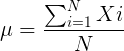
Xi, an observation on the i-th individual
Σ, or “sigma,” which instructs you to add them up (the X’s), from i = 1 (the first observation) to i = N (the last observation).
The sample mean,  , pronounced “eks bar,” of a collection of observations is given by
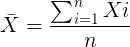
Note 1: Parameters (aka random variables) get Greek letters and sample variables get Roman letters. See Chapter 3.4
Weighted arithmetic mean.
In some cases you may have several samples from the same population. If the sample sizes are the same, you can calculate the average of averages without any fuss — just take all of the sample means and add them up, then divide by the total number of samples. If the sample sizes differ, then you needs to weight (W) each sample mean by its sample size. Simply divide each sample mean by its appropriate sample size, then add all of these up. That is the weighted average.
More generally, we can write
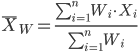
For example, consider a variable containing the following observations, for example, over the course of watching birds gathering at a drinking source (eg, recorded over 20 days, a single 5 minute interval per day), we can count how many times zero, one, two, etc birds are observed.
Table 1. A sample of counts of observations, eg, how many birds
| Observation | Frequency |
|---|---|
| 1 | 0 |
| 2 | 0 |
| 3 | 2 |
| 4 | 4 |
| 5 | 2 |
| 6 | 3 |
| 7 | 2 |
| 8 | 3 |
| 9 | 1 |
The observation “4” was observed four times; the observation “5” was observed twice, and so on for a total of 15 observations.
What is the arithmetic mean of these 15 observations? To solve this, well, you have a couple of choices. You could copy the numbers down as often as they appear and then calculate the mean in the usual way.
Other “means”.
The arithmetic average (illustrated above) is not the only way to estimate the mean.
The trimmed mean, also called the truncated mean, is a useful approach when data is widely dispersed — data spread away from the middle (see Chapter 3.3). Thus, the trimmed mean will be less influenced compared to the arithmetic mean by outlier data points, ie, data far from other data points in the set.
You would use the trimmed mean to describe the middle of a data set in which a plot shows most of the values are clumped together around a middle – and yet you see a few values that are much smaller or much greater. A specified percentage of the smallest and largest values are removed from the data set and then the simple arithmetic mean is calculated for the trimmed data set. For example, given a data set of daily rainfall for different cities, you might wish to remove the driest 5% and wettest 5% of the days in order to better compare the rainfall trends for the cities.
Calculating the trimmed mean is straight-forward in R: use the same built-in function, mean(), but add some options.
Note 2: This is a good time to remind you how to get help with R commands. Do you recall how to get help in R?
At the R prompt type
help(mean) or
?mean
The R Documentation page for mean() will pop up (assuming you allowed R to install help pages as html). Figure 1 shows a screenshot of a portion of the help page for mean()
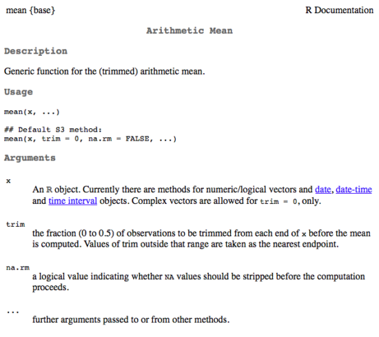
Figure 1. A portion of the R help page about the function mean.
From the help page (Fig 1) we can see that we can specify a trimmed mean by adding options to the mean(x, ...) command. For our x variable defined above, get the trimmed mean after 25% of the data are removed.
mean(x, trim=0.25)[1] 6From the help page we see that the only required option you need to feed the mean command is the name of the variable, in this case, “x” (it can be, of course, any name provided the data are attached). In this case we removed 25% of the values – 12.5% of the smallest values and 12.5% of the largest values – that’s also called the interquartile mean. We use a dot plot to show these trends (Fig 2).
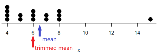
Figure 2. Dot plot of our x variable with locations of the mean (blue) and the trimmed mean (red). The Dotplot(x) function in package RcmdrMisc was used in Rcmdr to make this graphic. Arrows were added by hand. Dotplot() example code presented in Chapter 3.4.
If we recalculate a trimmed mean after dropping 10% of the points, or even 40% of the points, we get the same mean value of 6. The trimmed mean is an example of a robust estimator; it’s resistant to the influence of outliers.
Another useful descriptor of the middle is the geometric mean. The geometric mean is useful for calculating the average of ratios. Geometric mean would be used when you want to compare central tendency for different variables, each differing in scale. For example, gene expression results, reported as fold-changes, for different genes often shows tremendous differences among genes and would be best described by logarithmic scale, not arithmetic scale. Geometric mean expression values would be better choice for central tendency. Other examples are found in economics: for example, calculating compound interest or interest. The geometric mean applies whenever the scale is multiplicative and not additive
The geometric mean is given by the equation
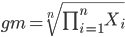
The geometric mean (gm) is equivalent to log-transforming your data, then calculating the arithmetic mean, and transforming the result back (with the antilog exponent.) As you recall, for our simple data set the arithmetic mean was 6.2. The geometric mean for this data was 5.977. Taking the natural log for each of the values from our simple data set, then calculating the arithmetic mean we have 1.788.
The antilog of this value is
exp(1.788)[1] 5.977Another frequently encountered mean is the harmonic mean, which is defined by the equation

Harmonic mean is appropriate for averaging rates. For example, what is the average speed traveled if you travel 30 miles per hour (mph) between point A and B, then on the return trip, your speed was 40 mph? If you think (30 + 40)/2 = 35 mph, then this would be incorrect — after all, the distance covered has not changed, just the time. The harmonic mean returns 34.2 mph. Let
y = c(30,40)The harmonic mean returns 34.2 mph ( see below “How to calculate these other means”)
Both harmonic and geometric means apply for values greater than zero.
How to calculate these “other” means.
In Microsoft Excel, calculate geometric mean via the function GEOMEAN(); calculate harmonic mean via the function HARMEAN().
The base R (and Rcmdr) doesn’t have built in functions for these, although you could download and install some R packages which do (eg, package psych, geometric.mean(variable), harmonic.mean(variable)). It is quicker to just to calculate these by submitting a snippet of code into the script window
For geometric mean of variable “x” at the R prompt type
exp(mean(log(x)))For harmonic mean of variable “x” at the R prompt type
1/mean(1/x)where is the base of the natural logarithm, Euler’s number, and log is the natural logarithm (in R, to get log to other bases you can use log10 for base 10 logarithm or log2 for base 2 logarithm, or log(x, base = n) for any base n of the variable x, and variable is the name of the variable you wish to do the calculations on.
R code: Do try on your own!
Here’s some numbers to try your hand. For example, create a variable containing a few numbers, any numbers. and write it to the variable named z
myZ = c(3,4,6,7,9,11,4)Now, calculate the arithmetic mean, the geometric mean, and the harmonic mean for the variable myZ. You should get Table 4.2)}
Table 2. Comparison of different means for myZ.
| mean | value |
|---|---|
| Arithmetic | 6.285714 |
| Geometric | 5.716403 |
| Harmonic | 5.204936 |
Try three more. In R (or R Commander script window), create three new variables.
varA = c(3,3,3,3)varB = c(1,2,3,12)varC = c(-3,0,1,3)Now, calculate the arithmetic mean, geometric mean, and harmonic mean for each variable.
For the simple arithmetic mean
mean(varA)For the geometric mean, use the formula above
exp(mean(log(varA)))For the harmonic mean, use the formula above
1/mean(1/varA)What did you get?
Other measures of central tendency
Median
The median, which lacks an accepted notation — we’ll go with  , divides a set of observed numbers into two equal halves. Half the observations are above the median, half of the observations are below the median. Arrange data from lowest to highest, take the middle measurement:

odd number of measurements minus the middle value minus even number of measurements minus average of the 2 middle values

Or, more succinctly, we have

To get the median in R type at the R prompt
median(variable)and of course, replace variable with the name of the variable containing the numbers. For our x variable created earlier, the function median returns in R
[1] 6[Note that the median for x was the same as the trimmed mean for x, which is consistent with with our view that the trimmed mean is a robust estimator of the middle of a data set.
Mode
Mode is another way to express the middle and it refers to the most frequent occurring measurement. Use of mode makes most sense for discrete or countable numbers. For a normal distribution, the mean, median and mode will be the same value. Note that a data set may have more than one mode. For example, what is the mode for the variable we created earlier?
myX = c(4,4,4,4,5,5,6,6,6,7,7,8,8,8,15)For this small data set we see that “4” is the most frequent with a count of four occurrences in the set.
Mode would seem like a straightforward function in R. However, it turns out there is not a mode function in the base package.
A little explanation is in order. In R, typing mode at the R prompt like so
mode(myX)returns
[1] "numeric" Not the answer we were expecting. In R, mode command is used to tell you what the mode (ie, way or manner in which some task is accomplished) of storage is for the variables.
In order to get the statistical mode we want, we either hunt down a package that contains mode estimation (eg, install the package DescTools use the Mode function — see below), or we can write a little code.
Note 3: A reminder — what we are attempting is to estimate a statistic. DescTools includes about 80 different statistics functions, including functions to calculate every statistic described in this chapter, chapter 3.3, and most other chapters in this book.
A quick Google search found a number of answers at stackoverflow.com (eg, question 2547402). The simplest response was to use names and max commands like so
temp = table(as.vector(myX))names (temp)[temp==max(temp)]Why the median may be a better middle than the mean
Comparing the two measures of central tendency can tell you without plotting how your data are distributed about the middle. Sample distributions are discussed in Chapter 6.
- When the distribution of the data is symmetric or normally distributed (discussed in Chapter 6.7) then the mean and the median will be about the same value
- When data are right-skewed (a few large values), then the mean will be greater than the median.
- When the data are left-skewed (a few small values), then the mean will be less than the median.
Here’s an illustration (Fig 3). I sampled 100 points from a random normal distribution with mean zero and standard deviation 0ne and another 100 points from a log-normal distribution also with mean zero and standard deviation one. In Figure 3, the histograms (see Chapter 4.2 – Histograms), along with summary statistics (see Note 4). Means are indicated with red arrows and medians are indicated with blue arrows.
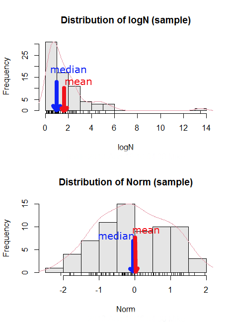
Figure 3. Normal and lognormal distributions with mean (red) and median (blue) noted for comparison.
So the median is a better descriptor or the central tendency of a sample distribution when the distribution is NOT normally distributed.
Note 4: “Summary statistics” refers to reporting of one or more descriptive statistics on a data set. The mean, median, standard deviation, range are common reported statistics. R Commander provides a menu to select from descriptive statistics, returning a table of the estimates. Rcmdr: Statistics → Summaries → Numerical summaries…
Scaling and transformation of data
Sometimes it is useful to standardize your data so that the variables all have the same scale. One algorithm for standardization is called normalization. Normalization implies that you correct the data so that data has a mean, μ, of zero, and a standard deviation, σ, of 1 (unit variance). There are several ways to standardize, each with strengths and limitations. To normalize we use the Z-score equation (see Chapter 6.7 for other uses of Z score).

where Xi is each observation in your data set.
Normalization will make outliers, the few points in a data set that are noticeably different from the central tendency of the rest of the data, smaller and less influential. When you normalize multiple sets of data, then each will have the same mean (0) and variance (unit variance), but the ranges will differ. An example of this is the simple product moment correlation — by standardizing you change the variances for the different variables to have the same unit variance.
As we will see later in class it is also useful to expand or contract the variability of the data or to change the shape of the distribution (if the data is not normally distributed). For example, if you compare individuals of a population for many morphological traits (eg body size, growth rate), the spread of points (called a distribution) will look more like a Poisson distribution (not symmetrical about the mean, a few individuals may be much larger…). This is partly due to the way in which morphological traits are measured. We normally measure body size on a linear scale (inches or centimeters). However, body size is affected by physiological processes that are more related to volume. Therefore, the more appropriate scale of measurement is on a log scale. We can transform the data measured on a linear scale to a log scale. For morphological traits this can produce a distribution that is normally distributed (bell shape). There are many more statistical procedures for data that is normally distributed than there are statistical procedures for Poisson distributions or any other type of distribution. Additional discussion about data transformation is introduced in Chapter 13.3.
You can always uncode or unstandardize your data after performing the statistical procedures and return to the original scale. In fact, when reporting descriptive statistics you should report the untransformed, uncoded data. Moreover, you will find it useful to report means adjusted for other variables (eg, from ANOVA or regression); if the ANOVA or regression equations are performed on transformed or coded data you would want to back calculate to the original scale after applying the ANOVA or regression adjustments. This advise will make more sense after we’ve discussed ANOVA (Chapter 12) and linear regression (Chapter 17).
R operators
The names command can be used to retrieve the names contained in the variable (if text types) or to set the names of the observations, which is what we are using it for here. We set the numbers to text names “4”, “5”, etc. then find the maximum count of named items in the temp table. The double equals operator (==) is used to tell R to find the object that is “equal to” something we specify, in this case, the max value (R Language Definition 2014). Table 3 shows common operators in R.
Table 3. Common arithmetic* and comparison** operators
| Operator | Description |
|---|---|
| ? | help |
| + | plus |
| - | minus |
| * | multiply |
| / | divide |
| : | series |
| > | greater than |
| < | less than |
| >= | greater than or equal to |
| <= | less than or equal to |
| = | left assignment |
| <- | left assignment |
== | equal to |
** To list and get help with use of comparison operators enter at the R prompt
help(Arithmetic)
help(Comparison)
The R package modeest has a number of algorithms for calculating the mode, depending on the kind of data you are working with. After installing the package and its dependencies, type at the R prompt
require(modeest)
mfv(myX)
[1] 4
Creating objects in R
Everything in R is an object (Chambers 2008). We provide many worked examples in Part 07. Working with your own data – Mike’s Workbook for Biostatistics. In brief, create a variable in R by assigning the vector x, either directly at the R prompt or in a script window (Rcmdr, RStudio), like so
myX = c(4,4,4,4,5,5,6,6,6,7,7,8,8,8,15)
The function c(), which stands for combine is used to combine the set of numbers into the object, myX. For small sets like this you may find it convenient to enter the values one by one and let R store it into the vector for you. For R installed on your computer, use the scan() function and your keyboard — scan() doesn’t work consistently in serverless R instances (eg., Google CoLab). Careful! Make sure that you remember to assign the results from scan to a vector.
I’ll create the object tryScan just to distinguish it from x, although I will enter the same values. Until R receives an interrupt signal from you, it will prompt you to enter numbers one row at a time. When you’ve reached the end, use the keyboard shortcut Ctrl + q (Windows) or Cmd + q (macOS) to interrupt keyboard input.
tryScan = scan()
1: 4
2: 4
3: 4
4: 4
5: 5
6: 5
7: 6
8: 6
9: 6
10: 7
11: 7
12: 8
13: 8
14: 8
15: 15
Read 15 items
tryScan
 [1] 4 4 4 4 5 5 6 6 6 7 7 8 8 8 15
The function tryScan is a very useful command, with many options, and can be used for more than keyboard entry. For example, you can paste from your computer’s clipboard a column of numbers from your spreadsheet.
R code calculate central tendency
Once we have the vectormyX, calculate the mean by entering at the R prompt
mean(myX)
and you should get the answer of 6.466667
And of course, you don’t type in the R prompt >, right?
Or, for the better option, create two variables, one containing the list of observed numbers and the second that contains the frequency for each observed number in the series. You would then use the command for weighted mean.
myY = c(4,5,6,7,8,15)
myW = c(4/15, 1/15, 3/15, 2/15, 4/15, 1/15)
Note — you can check that the frequencies sum to 1 by using the sum command like so
sum(myW)
For the weighted mean, the command is
weighted.mean(myY,myW)
and, the answer returned is 6.466667, the same as before.
There’s an R package for that.
We list code examples for all of the statistics described on this page, but as you can imagine, there are packages that include these and other useful functions, or “wrapper functions” that make writing code easier in R. A good example is the DescTools package. One advantage of using a package like DescTools is that it cuts through the need to remember specific commands for basic data exploration. For example, just call the Desc() function to yield several measures of central tendency and dispersion (see Chapter 3.3).
The R code and output follows, along with a plot (Fig 4). The mean and median are highlighted in orange.
Desc(myX)
────────────────────────────────────────────────────────────────────────────────
myX (numeric)

length      n   NAs unique   0s  mean meanCI'
    15     15     0      6    0  6.47    4.92
       100.0%  0.0%        0.0%          8.02

   .05    .10   .25 median  .75   .90     .95
  4.00   4.00  4.50   6.00 7.50  8.00   10.10

range      sd vcoef    mad  IQR  skew    kurt
11.00    2.80  0.43   2.97 3.00  1.72    2.94

  value freq   perc cumfreq cumperc
1     4    4  26.7%       4   26.7%
2     5    2  13.3%       6   40.0%
3     6    3  20.0%       9   60.0%
4     7    2  13.3%      11   73.3%
5     8    3  20.0%      14   93.3%
6    15    1   6.7%      15  100.0%

' 95%-CI (classic)

Figure 4. Histogram, box plot, and cumulative distribution function plot generated by default by Desc() call.
Lots of output! This is a good example of how to explore data — describe the middle (eg, mean and median), but also the variability about the middle (eg, range, standard deviation — sd, mean absolute deviation — mad, coefficient of variation — vcoef), and distribution shape (quantiles — 0.05, 0.25 etc, kurt, skew). The plots — histogram, box plot, and cumulative distribution plots — are explained in Chapter 4.
Use aggregate() to calculate summary statistics by group.
So far, all code presumes need to calculate descriptive statistics one vector at a time. In general, we need summary statistics for more than one group or strata. For example, we may ask, what are the average body temperature readings measured by IR device on different body areas from several subjects (question 8a, Homework 2A: Descriptive statistics in Mike’s Workbook for Biostatistics).
The aggregate() function in R simplifies calculating means by groups by providing a concise and efficient way to apply a summary function (like mean()) to a variable, grouped by one or more other variables. The format for aggregate is
aggregate(x = variable_to_aggregate ~ grouping_variable, FUN = mean, data = your_dataframe)
Questio8a had two levels of body regions, “Forehead” and “Throat.” Assuming the variable is named bodyTemp and the grouping variable is called bodyGroup and stored in the attached data.frame question08a, then the following R code provides the requested summary statistics by groups.
aggregate(bodyTemp ~ bodyGroup, data = question08a,
function(x) c(mean = mean(x)))
Additional statistics can be requested by adding one after the other following mean(x), eg, median = median(x).
Note 5: aggregate() is part of the base R installation. Additional functions are available, including dplyr and data.table packages, which the user is encouraged to explore!
The advantage of use of R Commander, it’s easy to get multiple statistics by groups by following the drop down menus, beginning with Statistics > Summaries > Table of statistics… (Fig 5).

Figure 5. Screenshot R Commander, summary statistics by group.
Questions
- Find the help page in R for the median function. How does the function handle missing values?
- For a simple data set like the following
myY <- c(1,1,3,6)you should now be able to calculate, by hand, the
• mean • median • mode - If the observations for a ratio scale variable are normally (symmetrically) distributed, which statistic of central tendency is best (eg, less sensitive to outlier values)?
- In the
names()command, what do you think the result will be if you replacemaxin the command withmin? - If data are right skewed, what will be the order of the mean, median, and mode?
- Body mass of Rhinella marina (formerly Bufo marinus, Fig 6),
bufo <- c(71.3, 71.4, 74.1, 85.4, 85.4, 86.6, 97.4, 99.6, 107, 115.7, 135.7, 156.2)

Figure 6. Female Rhinella marina (formerly Bufo marinus), Chaminade University campus. Body length 23.5 cm. Click image to view full sized image.
- Under what circumstances is it appropriate to transform raw data?
- What does “standardize” or “normalize” imply as actions to take with data?
Quiz Chapter 3.2
Measures of Central Tendency
Chapter 3 contents
- Exploring data
- Data types
- Measures of Central Tendency
- Measures of dispersion
- Estimating parameters
- Statistics of error
- References and suggested readings