19.2 – Bootstrap sampling
Introduction
Bootstrapping is a general approach to estimation or statistical inference that utilizes random sampling with replacement (Kulesa et al. 2015). In classic frequentist approach, a sample is drawn at random from the population and assumptions about the population distribution are made in order to conduct statistical inference. By resampling with replacement from the sample many times, the bootstrap samples can be viewed as if we drew from the population many times without invoking a theoretical distribution. A clear advantage of the bootstrap is that it allows estimation of confidence intervals without assuming a particular theoretical distribution and thus avoids the burden of repeating the experiment.
Base install of R includes the boot package. The boot package allows R users to work with most functions, and many authors have provided helpful packages. I highlight a couple packages
install packages lmboot, confintr
Example data set, Tadpoles from Chapter 14, copied to end of this page for convenience (scroll down or click here).
Bootstrapped 95% Confidence interval of population mean
Recall classic frequentist (large-sample) approach to confidence interval estimates of mean by R
x = round(mean(Tadpole$Body.mass),2); x
n = length(Tadpole$Body.mass); n
s = sd(Tadpole$Body.mass); s
error = qt(0.975,df=n-1)*(s/sqrt(n)); error
lower_ci = round(x-error,3)
upper_ci = round(x+error,3)
paste("95% CI of ", x, " between:", lower_ci, "&", upper_ci)
Output results are
> n = length(Tadpole$Body.mass); n
[1] 13
> s = sd(Tadpole$Body.mass); s
[1] 0.6366207
> error = qt(0.975,df=n-1)*(s/sqrt(n)); error
[1] 0.384706
> paste("95% CI of ", x, " between:", lower_ci, "&", upper_ci)
[1] "95% CI of 2.41 between: 2.025 & 2.795"
We used the t-distribution because both  the population mean and
 the population standard deviation were unknown. Thus, 95 out of 100 confidence intervals would be expected to include the true value.
Bootstrap equivalent
library(confintr)
ci_mean(Tadpole$Body.mass, type=c("bootstrap"), boot_type=c("stud"), R=999, probs=c(0.025, 0.975), seed=1)
Output results are
Two-sided 95% bootstrap confidence interval for the population mean based on 999 bootstrap replications
and the student method

Sample estimate: 2.412308
Confidence interval:
    2.5%    97.5%
2.075808 2.880144
where stud is short for student t distribution (another common option is the percentile method — replace stud with perc), R = 999 directs the function to resample 999 times. We set seed=1 to initialize the pseudorandom number generator so that if we run the command again, we would get the same result. Any integer number can be used. For example, I set seed = 1 for output below
Confidence interval:
    2.5%    97.5%
2.075808 2.880144
compared to repeated runs without initializing the pseudorandom number generator:
Confidence interval:
    2.5%    97.5%
2.067558 2.934055
and again
Confidence interval:
    2.5%    97.5%
2.067616 2.863158
Note that the classic confidence interval is narrower than the bootstrap estimate, in part because of the small sample size (i.e., not as accurate, does not actually achieve the nominal 95% coverage). Which to use? The sample size was small, just 13 tadpoles. Bootstrap samples were drawn from the original data set, thus it cannot make a small study more robust. The 999 samples can be thought as estimating the sampling distribution. If the assumptions of the t-distribution hold, then the classic approach would be preferred. For the Tadpole data set, Body.mass was approximately normally distributed (Anderson-Darling test = 0.21179, p-value = 0.8163). For cases where assumption of a particular distribution is unwarranted (e.g., what is the appropriate distribution when we compare medians among samples?), bootstrap may be preferred (and for small data sets, percentile bootstrap may be better). To complete the analysis, percentile bootstrap estimate of confidence interval are presented.
The R code
ci_mean(Tadpole$Body.mass, type=c("bootstrap"), boot_type=c("perc"), R=999, probs=c(0.025, 0.975), seed=1)
and the output
Two-sided 95% bootstrap confidence interval for the population mean based on 999 bootstrap replications
and the percent method
Sample estimate: 2.412308
Confidence interval:
    2.5%    97.5%
2.076923 2.749231
In this case, the bootstrap percentile confidence interval is narrower than the frequentist approach.
Model coefficients by bootstrap
R code
Enter the model, then set B, the number of samples with replacement.
myBoot <- residual.boot(VO2~Body.mass, B = 1000, data = Tadpoles)
R returns two values:
bootEstParam, which are the bootstrap parameter estimates. Each column in the matrix lists the values for a coefficient. For this model,bootEstParam$[,1]is the intercept andbootEstParam$[,2]is the slope.origEstParam, a vector with the original parameter estimates for the model coefficients.seed, numerical value for the seed; use seed number to get reproducible results. If you don’t specify the seed, then seed is set to pick any random number.
While you can list the $bootEstParam, not advisable because it will be a list of 1000 numbers (the value set with B)!
Get necessary statistics and plots
#95% CI slope
quantile(myBoot$bootEstParam[,2], probs=c(.025, .975))
R returns
    2.5%    97.5%
335.0000 562.6228
#95% CI intercept
quantile(myBoot$bootEstParam[,1], probs=c(.025, .975))
R returns
     2.5%     97.5%
-881.3893 -310.8209
Slope
#plot the sampling distribution of the slope coefficient
par(mar=c(5,5,5,5)) #setting margins to my preferred values
hist(myBoot$bootEstParam[,2], col="blue", main="Bootstrap Sampling Distribution",
xlab="Slope Estimate")
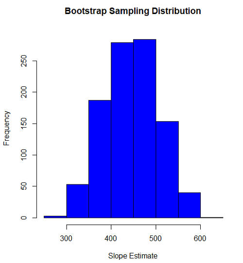
Figure 1. histogram of bootstrap estimates for slope
Intercept
#95% CI intercept
quantile(myBoot$bootEstParam[,1], probs=c(.025, .975))
par(mar=c(5,5,5,5))
hist(myBoot$bootEstParam[,1], col="blue", main="Bootstrap Sampling Distribution",
xlab="Intercept Estimate")
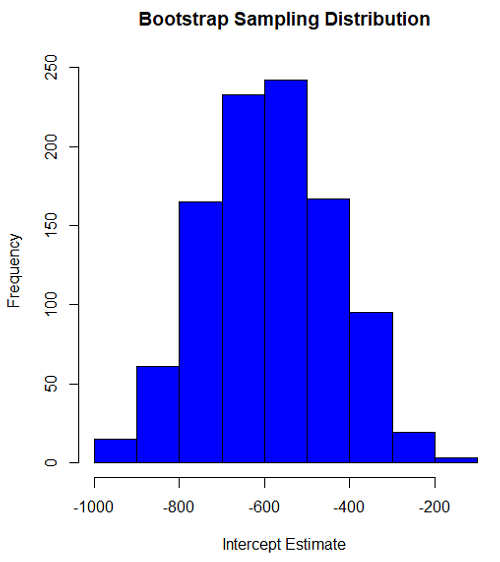
Figure 2. Histogram of bootstrap estimates for intercept.
Questions
edits: pending
Data set used this page (sorted)
| Gosner | Body mass | VO2 |
| I | 1.76 | 109.41 |
| I | 1.88 | 329.06 |
| I | 1.95 | 82.35 |
| I | 2.13 | 198 |
| I | 2.26 | 607.7 |
| II | 2.28 | 362.71 |
| II | 2.35 | 556.6 |
| II | 2.62 | 612.93 |
| II | 2.77 | 514.02 |
| II | 2.97 | 961.01 |
| II | 3.14 | 892.41 |
| II | 3.79 | 976.97 |
| NA | 1.46 | 170.91 |
Chapter 19 contents
- Introduction
- Jackknife sampling
- Bootstrap sampling
- Monte Carlo methods
- Ch19 References and suggested readings
20.1 – Area under the curve
Introduction.
The classical physiological area under the curve, AUC, represents the total change in  given change in
 . For example, if is time, and is oxygen consumption — eg, respirometry: recorded as an analog voltage output (millivolts or volts) from a gas analyzer to a data acquisition (DAQ) board — an AUC would be appropriate to quantify the total oxygen consumption following strenuous exercise (Excess post-exercise oxygen consumption, EPOC) or following a large meal (Specific Dynamic Action, SDA). The area represents the total, cumulative volume of oxygen consumed over that specific timeframe, eg, calculating an individual’s total EPOC.
In machince learning, the axes are probabilities and error rates. The area tells you how accurate a decision-making model is. We plot True Positive Rate (Sensitivity) against False Positive Rate (1 – Specificity) across every possible mathematical decision threshold (from 0% to 100% confidence). The curve now represents the shifting balance between catching true positives and committing false positives and the area summarizes how cleanly the model separates two distinct classes, eg, Sick vs. healthy. An area of 1.0 means perfect separation with zero overlap.
Area under the relative (receiver) operating carrier, AUROC, shows characteristics of a diagnostic model, a graphic used to show trade off between sensitivity and specificity. Classifier performance. Used to find the appropriate cut-off. Plot true positive rates against false positive rates as cumulative functions, shows the relationship between sensitivity and specificity for every possible cut off value. Can then calculate AUC to get a measure of the intervention’s ability to discriminate between true and false positive rates.
Related, area under precision-recall curve, AUPRC, is a single scalar metric that measures a binary classification model’s ability to balance precision (how many predicted positives are actually positive) and recall (how many actual positives are caught) across all possible decision thresholds. Here, precision and recall refer to both the accuracy of the model’s positive predictions and its ability to find all the positive cases.
From Chapter 7 we defined
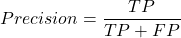
where  is true positives and
 is false positives.
We now introduce recall, which is also refered to as sensitivity
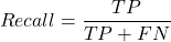
Precision measures the quality of your model’s positive guesses; Recall measures how many actual positive cases in the dataset were identified by the model.
AUC evaluates a model’s ability to distinguish between both and equally, while AUPRC focuses strictly on the model’s performance regarding the positive (rare) class.
AUC would be preferred when your dataset is balanced (equal positives and negatives) OR when you care equally about performance on both classes. For example, dataset of patients with flu or Covid from a clinic during winter months where there is roughly balanced 50/50 split of patients presenting with either Flu or Covid. You want a model that accurately classifies both which favors AUC approach.
AUPRC would be the choice when your dataset is highly imbalanced, ie, the positive class is rare. In contrast, AUPRC would be favored for scenarios where a researcher is screening 100,000 asymptomatic patients for a rare disease that only 10 people actually have.
Physiology Area under the curve
Download and install R package MESS; requires geepack, geeM, and Matrix packages
R code
x <- seq(1:10)
y <- c(1,4,5,2,11,22,9,7,5,1)
#length(x)==length(y)
#smooth the data
loxy <- loess(y~x)
#Make a plot (Fig. 1)
plot(x,y, pch=19, cex=2, col="blue")
lines(predict(loxy), type="l", col="red")
where == is an R comparison operator.
And R output
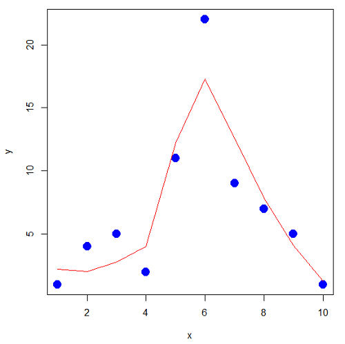
Figure 1. Area under the curve example.
library(MESS)
auc(x,y,from=0,rule=2)
auc(x,loxy$fitted,from=0,rule=2)
And R output
#area under curve for raw data
[1] 67
#area under curve for smoothed data
[1] 66.77616
Machine Learning area under the curve.
# Install and load the ROCR package if you haven't already
# install.packages("ROCR")
# modified from https://rviews.rstudio.com/2019/03/01/some-r-packages-for-roc-curves/

library(ROCR)
df <- data.frame(ROCR.simple)
pred <- prediction(df$predictions, df$labels)
perf <- performance(pred,"tpr","fpr")

# 1. Calculate the actual numeric AUC value
auc_perf <- performance(pred, "auc")
auc_value <- round(unlist(auc_perf@y.values), 4)

# 2. Plot the ROC curve with colorized thresholds and custom labels
plot(perf,
colorize = TRUE,
main = "ROC Curve",
xlab = "False Positive Rate (1 - Specificity)",
ylab = "True Positive Rate (Sensitivity)")

# 3. Add the AUC value as a subtitle
mtext(paste("AUC =", auc_value), side = 3, line = 0.5)

# 4. Add a diagonal 50/50 reference line
abline(a = 0, b = 1, lty = 2, col = "darkgray")
End R code.
Note 1. I mostly provide S3 R code examples in this eBook. In R, the @ symbol is used to extract a specific piece of data (called a slot) from an S4 object. It works almost exactly like the $ sign, but while $ is used for basic lists or standard data frames (S3 objects), @ is reserved strictly for the more structured, formal object system in R known as S4.
R output.
The calculated AUC was  . The right-hand axes are color codes by AUC values (Fig 2): good tests AUC between 0.8 and 0.9, very good tests greater than 0.9.
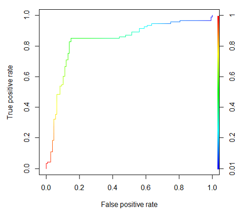
Figure 2. Example ROC curve.
Area under the precision recall curve
AUPRC measures the overall performance of a binary classification model by summarizing how well it balances precision and recall across all possible decision thresholds. A score closer to 1.0 means the model is very good at finding real positive cases without making many mistakes, which is especially useful when your dataset has very few positive examples. A score closer to 1.0 means the model is very good at finding real positive cases without making many mistakes.
R code.
library(ROCR)

# 1. Prepare data and prediction object
df <- data.frame(ROCR.simple)
pred <- prediction(df$predictions, df$labels)

# 2. Extract Precision and Recall for the plot
perf_pr <- performance(pred, measure = "prec", x.measure = "rec")

# 3. Calculate the numeric AUPRC value
# In ROCR, AUPRC is calculated by finding the Area Under the Precision/Recall curve ("aucpr")
perf_auprc <- performance(pred, measure = "aucpr")
auprc_value <- round(unlist(perf_auprc@y.values), 4)

# Print the final AUPRC score to the console
cat("The calculated AUPRC is:", auprc_value, "\n")

# 4. Plot the Precision-Recall Curve using base R graphics
plot(perf_pr,
colorize = TRUE,
main = paste("Precision-Recall Curve (AUPRC =", auprc_value, ")"),
xlab = "Recall (Sensitivity)",
ylab = "Precision (Positive Predictive Value)")
End R code.
R output.
The calculated AUPRC was  .
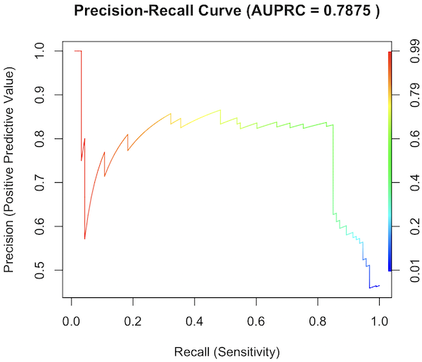
Figure 3. Precision recall curve.
The differences: AUC evaluates how well the model separates both classes equally, while AUPRC evaluates how reliably the model handles the positive class alone.
The Interpretive baselines:
- Figure 2: AUC Baseline is always 0.5. A completely random model yields a diagonal line from (0,0) to (1,1), resulting in an AUC of 0.5. This baseline never changes, regardless of how rare your disease is.
- Figure 3: AUPRC Baseline depends on prevalence. A random model yields a flat horizontal line across the plot. The height of this line equals the proportion of positive cases in your dataset (
 ). If only 1% of the patients have a rare condition, a random model’s AUPRC baseline is 0.01.
What a shifting threshold means:
- On an AUC Curve: As you lower your decision threshold to catch more sick people, you track how fast your True Positive Rate rises compared to your False Positive Rate. You are looking at the overall trade-off between the entire healthy population and the entire sick population.
- On an AUPRC Curve: As you lower your threshold to catch more sick people, you track Recall against Precision. This evaluates the quality of the “Positive” alerts. It directly measures how quickly the pool of patients you flagged as “high risk” becomes diluted with false alarms.
References and suggested readings
Çorbacıoğlu, Ş. K., & Aksel, G. (2023). Receiver operating characteristic curve analysis in diagnostic accuracy studies: A guide to interpreting the area under the curve value. Turkish Journal of Emergency Medicine, 23(4), 195–198.
Lobo, J. M., Jiménez-Valverde, A., & Real, R. (2008). AUC: A misleading measure of the performance of predictive distribution models. Global Ecology and Biogeography, 17(2), 145–151.
Martin, B., Bennett, T. D., DeWitt, P. E., Russell, S., & Sanchez-Pinto, L. N. (2025). Use of the Area Under the Precision-Recall Curve to Evaluate Prediction Models of Rare Critical Illness Events. Pediatric Critical Care Medicine, 26(6), e855–e859.
Ozenne, B., Subtil, F., & Maucort-Boulch, D. (2015). The precision–recall curve overcame the optimism of the receiver operating characteristic curve in rare diseases. Journal of Clinical Epidemiology, 68(8), 855–859. https://doi.org/10.1016/j.jclinepi.2015.02.010
Steyerberg, E. W., & Vergouwe, Y. (2014). Towards better clinical prediction models: Seven steps for development and an ABCD for validation. European Heart Journal, 35(29), 1925–1931.
Questions
- Write up three learning outcomes for this page. Hint: Point your favorite generative AI to this page and ask for help
Chapter 20 contents
- Additional topics
- Area under the curve
- Peak detection
- Baseline correction
- Surveys
- Time series
- Dimensional analysis
- Estimating population size
- Diversity indexes
- Survival analysis
- Growth equations and dose response calculations
- Plot a Newick tree
- Phylogenetically independent contrasts
- How to get the distances from a distance tree
- Binary classification
- Meta-analysis
/MD
6.5 – Discrete probability distributions
Binomial distribution
Discrete refers to particular outcomes — data that take on only specific separate values. Discrete data types include all of the categorical types we introduced earlier, including binary, ordinal, and nominal.
The binomial probability distribution is a discrete distribution for the number of successes, k, in a sequence of n independent trials, where the outcome of each trial can take on only one of two possible outcomes. For cases of 0 or 1, yes or no, “heads” or “tails,” male or female, pass or fail, we talk about the binomial distribution, because the outcomes are discrete and there can be only two possible (binary) outcomes.
Note 1: The biological definition of sex is binary — whether sexually reproducing organism produces male (sperm) or female (ovum) gametes (cf discussion in Goymann et al 2022). For the argument that sex is a continuum held by some biomedical and social scientists, see Ainsworth 2015.
The mathematical function of the binomial is written as

where the binomial coefficient is given by
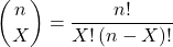
and X refers to the number of ways to choose “success” from n observations.
Consider an example.
We have to define what we mean by success. For coin toss, this might be the number of heads.
The mean for the binomial this is given simply as

where X is “Heads” (the category of successes for our example), and p corresponds to the probability the selected event occurs, in this case, “Heads.”
The variance of the binomial distribution is given by

Here’s a density plot of two trials with success 2% with n (x) equal to 20 (Fig 1).
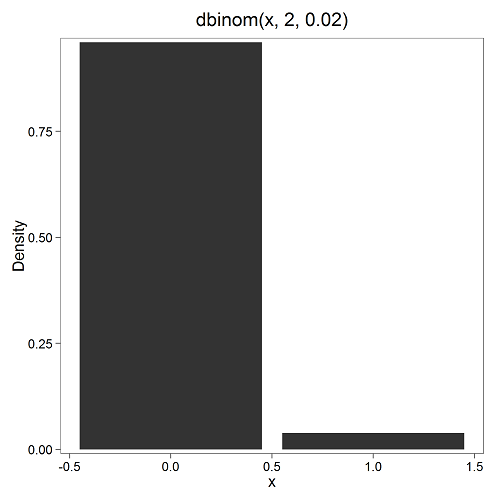
Figure 1. Plot generated with KMggplot2 Rcmdr plugin.
Here’s the R code
Create the trials, 1 through 20, then create an object to hold the number of trials
nSize=1:20
Size <- length(nSize); Size
R returns
[1] 20
Assign the probability value to an object
prob <- 0.02
Next, calculate the mean, mu, and the variance, var, for the binomial with prob = 0.02 and number of trials Size = 20
mu <- Size*prob
var <- Size*prob*(1-prob)
Print the mean and variance; lets assign them to an object then print the object
stats <- c(mu, var); stats
And R returns
[1] 0.400 0.392
And here’s a real-world example. Twinning in humans is rare. In Hawaiʻi in the 1990’s the rate of twin births (monozygotic and dizygotic) was about 20 for every 1000 births or 2%. “Success” here then is twin births.
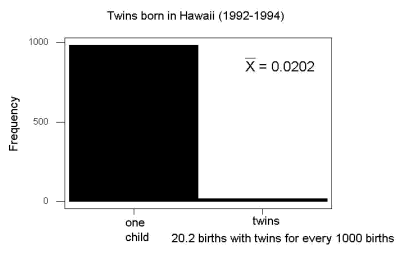
Figure 2. Example of binomial-like distribution: reported twins born in Hawaiʻi.
Interestingly, rates of twins have since increased in Hawaiʻi (31 out of 1000 births) and in the United States overall (33 out of 1000 births) (Table 2, NCHS Data Brief No. 80, 2012). Data for Fig 2 were for year 2009.
Out of ten births, what is the probability of two twin births in Hawaiʻi?

You can solve this with your calculator (yikes!), or take advantage of online calculators (GraphPad QuickCalcs), or use R and Rcmdr.
In R, simply type at the prompt
dbinom(2,10,0.031)
[1] 0.03361446
Try in R Commander.
Rcmdr → Distributions → Discrete distributions → Binomial distribution → Binomial probabilities …

Figure 3. Rcmdr menu to get binomial probability.
Note I used p = 0.033 the rate for entire USA. Here’s the output
> .Table <- data.frame(Pr=dbinom(0:10, size=10, prob=0.033))
> rownames(.Table) <- 0:10
> .Table
Pr
0  7.149320e-01
1  2.439789e-01
2  3.746728e-02 ← Answer, 0.0375 or 3.75%
3  3.409639e-03
4  2.036263e-04
5  8.338782e-06
6  2.371422e-07
7  4.624430e-09
8  5.918028e-11
9  4.487991e-13
10 1.531579e-15
And here is the output for our example from Hawaiʻi (p = 0.031).
> .Table <- data.frame(Pr=dbinom(0:10, size=10, prob=0.031))
> rownames(.Table) <- 0:10
> .Table
Pr
0  7.298570e-01
1  2.334940e-01
2  3.361446e-02 ← Answer, 0.0336 or 3.36%
3  2.867694e-03
4  1.605494e-04
5  6.163507e-06
6  1.643178e-07
7  3.003893e-09
8  3.603741e-11
9  2.561999e-13
10 8.196283e-16
We use the binomial distribution as the foundation for the binomial test, ie, the test of an observed proportion against an expected population level proportion in a Bernoulli trial.
Hypergeometric distribution
The binomial distribution is used for cases of sampling with replacement from a population. When sampling without replacement is done, the hypergeometric distribution is used. It is the number of successes, k, in a sequence of n independent trials drawn from a fixed population.
Note 2: A fixed population in epidemiology refers to a group of individuals, defined by set of characteristics. Examples include individuals selected because they all share a common life event, eg, giving birth. The population is “fixed” because, once an individual is included in the population, they remain a member of the population even if their characteristics change during the duration of the study. The opposite of a fixed population is an dynamic or open population. Definitions from Chapter 2 in Aschengrau and Seage (2003).
This sampling scheme means that each draw is no longer independent — with each draw you decrease the remaining number of observations and thus change the proportion.
The P-value from the hypergeometric distribution is often used to study if genes from a list of Gene Ontology (eg, biological process functional terms like “cell cycle,” or “apoptosis”) are enriched in the sets of genes with expression differences across the treatment groups (cf, discussion in Cao and Zhang 2014). The R package gprofiler2, which links to a Cloud service at g:Profiler, the can be used to do gene enrichment analyses with stunning visualizations (eg, Manhattan plot) suitable for publication.
The mathematical function of the hypergeometric is written as

where N is the population size, K is the number of successes in that population, and n and k are defined as above. Lets look apply this to the twinning problem.
In 2009, 2200 women gave birth in Hawaiʻi County, Hawaiʻi. Out of 10 births, what is the probability of 2 twin births in Hawaiʻi?
Assuming “risk” of twinning is the same rate as in rest of USA, then we have expected 72 successes in this population (0.033 * 2200).
Here’s the graph (Fig 4).
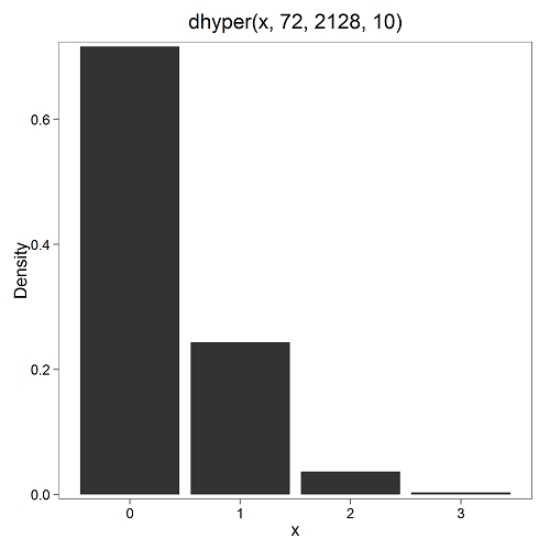
Figure 4. Plot of hypergeometric distribution twinning Hawaiʻi.
where the X axis values shows the number of events with successes (twin births). Taking the bin 2 (we wanted to know about probability of 2 out of ten), we can draw a line back to the Y-axis to get our probability — looks like about 5% roughly. Plot drawn with KMggplot2
To get the actual probability,
Rcmdr → Distributions → Discrete distributions → Hypergeometric distribution → Hypergeometric probabilities …

Figure 5. Rcmdr menu to get hypergeometric probability.
where m is the number of successes, n is the number of “failures,” and k is the number of trials.
> .Table
Pr
0 0.716453457
1 0.243438645
2 0.036688041 ← Answer, 0.0367 or 3.67%
3 0.003228871
The reference to white and black balls and urns is a device described by Bernoulli himself and has been used by others ever since to discuss probability problems (called the urn problem) and so I apply it here to be consistent. The urn contains a number of white (x) and a number of black (y) balls mixed together. One ball is drawn randomly from the urn — what color is it? The ball is then is either returned into the urn (replacement) or it is left out (without replacement) as in the hypergeometric problem, and the selection process is repeated.
Besides applications in gambling and balls-in-urns problems, this distribution is the basis for many tests of gene enrichment from microarray analyses. The hypergeometric forms the basis of the Fisher Exact test (see Chapter 9.5).
Discrete uniform distribution
For discrete cases of “1,” “2,” “3,” “4,” “5,” or “6,” on the single toss of fair dice, we can talk about the discrete uniform distribution because all possible outcomes are equally likely. If you are branded as a “card-counter” in Las Vegas, all you’ve done is reached an understanding of the uniform distribution of card suits!
One biological example would be the fate of a random primary oocyte in the human (mammal) female — three out of four will become polar bodies, eventually reabsorbed, whereas one in four will develop into a secondary oocyte (egg); the uniform distribution has to do with the counts of the products — each of the four primary oocytes has the same (apparently) chance (25%) of becoming the egg (Edwards and Beard 1997).
Analyses in biological research often use a uniform distribution as a baseline or null model (Gotelli and Ulrich 2011). For DNA sequencing, the uniform distribution provides a baseline for assessing coverage bias, eg, GC bias (Ross et al 2013). The uniform distribution underlies the Jukes–Cantor evolutionary model. The Jukes–Cantor model assumes equal substitution rates among all four nucleotides (A, T, C, G) and equal base frequencies (Felsenstein 2003).
The uniform distribution exists also for continuous data types, where every value within a specified interval has equal probability density. For example, DNA shearing — by endonucleases, proteases, or tansposases — during initial library prep for sequencing reactions, breakpoints may be modeled as uniformly distributed along fragment length. Non-uniform distributions reveal cleavage bias. Sequence-dependent cleavage bias is concluded when certain DNA fragments or sequences are generated or detected more (or less) frequently than would be expected by chance (Meyer and Liu 2014). This generates many false positives — that is, identifying a biological signal or molecule that isn’t actually there (Nix et a; 2008).
Poisson distribution
An extension from the binomial case is that, rather than following success or failure, you may have the following scenario. Consider a wind-dispersed seed released from a plant. If we markup the area around the plant in grids, we could then count the number of seeds within each grid. Most grids will have no seeds, some grids will have one seed, a few grids may have two seeds, etc. Multiple seeds in grids is a rare event. The graph might look like
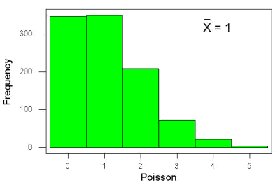
Figure 6. Example, poisson-like graph: the number of wind-dispersed seeds within each grid.
In molecular biology, use of Poisson distribution is common. In digital PCR for example, a DNA sample is diluted and divided into thousands of small reaction volumes or partitions. Thus, each partition contains either zero molecules, one molecule, or more than one molecule, where the loading of molecules into partitions is assumed to be independent, random, and rare per partition. In sequencing, Poisson models are used to describe random sampling of molecules and reads, especially when coverage is generated by non-deterministic processes like shotgun sequencing.
The Poisson has interesting properties, one being that the expected mean, λ, is equal to the variance. Lambda is, with respect to the Poisson distribution, the average number of times an event happens over a specific period or area.
An equation is

where μ is the mean (or could substitute with variance!), e is the natural logarithm, and X is number of successes you are interested in. For example, if μ = 1, what is the probability of observing a grid with five seeds? Simple enough to do this by hand, but let’s use Rcmdr instead. Here’s the graph (Fig 7) from Rcmdr (KMggplot2 plugin).
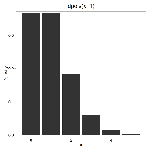
Figure 7. The probability of observing a grid with five seeds, poisson μ = 1 (ggplot2).
and for the actual probability we have from R
dpois(5, lambda = 1)
[1] 0.003065662
Rcmdr → Distributions → Discrete distributions → Poisson distribution → Poisson probabilities … (Fig 8)
The only thing to enter is the mean (some call μ lambda with symbol λ).
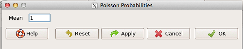
Figure 8. Rcmdr menu, poisson probability.
Here’s the output from R. For intervals 0, 1, 2, 3, …, 6 (Rcmdr just enters this range for you!
> .Table <- data.fram(Pr=dpois(0:6, lambda = 1))
> rownames(.Table) <- 0:6
> .Table
Pr
0 0.3678794412
1 0.3678794412
2 0.1839397206
3 0.0613132402
4 0.0153283100
5 0.0030656620 ← Answer, 0.0307 or 3.07%
6 0.0005109437
Next — Continuous distributions
And finally, for ratio (continuous) scale data, which can take on any value, we can express the chance that probability of a given point as a continuous function, with the normal distribution being one of the most important examples (there are others, like the F-distribution). Many statistical procedures assume that the data we use can be viewed as having come from a “normally distributed population.” See Chapter 6.6.
Questions
1.2. Quarterback sacks by game for the NFL team Seahawks, years 2011 through 2022 are summarized below (data extracted from https://www.pro-football-reference.com/ ).
| Sacks | How many games? |
| 0 | 25 |
| 1 | 46 |
| 2 | 49 |
| 3 | 39 |
| 4 | 25 |
| 5 | 14 |
| 6 | 8 |
| 7 | 2 |
| 8 | 1 |
| 9 | 0 |
a) Assuming a Poisson distribution, what are the mean (lambda) and variance?
b) The table covers a total of 112 games. How many sacks (events) were observed?
c) What is the probability of the Seahawks getting zero sacks in a game (in 2022, a season was 17 games; prior years a season was 16 games)?
Quiz Chapter 6.5
Discrete probability
Chapter 6 contents
- Introduction
- Some preliminaries
- Ratios and proportions
- Combinations and permutations
- Types of probability
- Discrete probability distributions
- Continuous distributions
- Normal distribution and the normal deviate
- Moments
- Chi-square distribution
- t distribution
- F distribution
- References and suggested readings
6.3 – Combinations and permutations
Introduction
In statistical inference, an important foundational skill is to be able to count the possible outcomes of an experiment — the sample space. For example, when drawing on a sample of individuals for study from specific groups (strata) of a population, combinations may be calculated; where it is unwarranted to assume a particular theoretical probability distribution applies, permutation tests create a reference distribution by calculating all possible values of a test statistic under rearrangements of the observed data.
The simplest place to begin with probability is to define an event — an event is an outcome — a “Heads” from a toss of coin, or the chance that the next card dealt is an ace in a game of Blackjack. In these simple cases we can enumerate how likely these events are given a number of chances or trials. For example, if the coin is tossed once, then the coin will either land “Heads” or “Tails” (Fig 1).
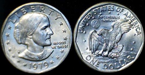
Figure 1. Heads (left) and Tails (right) of a USA Susan B. Anthony dollar.
We can then ask what is the likelihood of ten “Heads” in ten tosses of a fair coin?
And this gets us to some basic rules of probability:
- if successive events are independent, then we multiply the probability
- if events are not independent, then the probability adds
- do we sample without replacement, ie, an object can only be used once?
- do we sample with replacement, ie, an object gets placed “back in the deck” and can be used again and again
Combinations and Permutations
Both combinations and permutations pertain to how samples are selected from a population. Combinations are used if the events or objects of the sample are all of the same kind, whereas for permutations, it is implied that the events or objects are not all of the same kind.
Figure 2. A combination lock
Combinations ignore the order of the events; permutations are ordered combinations. For replacement, the formula for permutations is simply 
In the case of the ten “Heads,” in ten successive trials, the probability is  “ten-times” or
 = 0.0009766 (in R, just type
0.5^10 or (1/2)^10 at the R prompt).
Examples of permutations in biology include,
Given the four nucleotide bases of DNA, adenine (A), cytosine (C), guanine (G), and thymine (T), how many codons are possible?

where the three (3) refers to the codon, three nucleotide genetic code. Codons are trinucleotide sequences of DNA or RNA that correspond to a specific amino acid. For transcription initiation of a protein-coding gene, a key sequence must be present in the promoter region of the gene. In Archaea and Eukaryotes, that sequence is called the TATA box. How often do we expect to find by chance the heptamer (ie, seven bases) TATA box sequence in the human genome?
Note 1: The consensus TATA box sequence, TATAWAW (W can be either Adenine or Thymine, per Standard IUB/IUPAC nucleic acid code). The TATA box is the binding site for transcription factors, particularly the TATA binding protein.

Thus, we would expect at random to find TATA box sequences every 16,384 bases along the genome. For the human genome of 3.3 billion bases then we would expect at random more than 200,000 TATA box consensus sequences.
Another way to put this is to ask how many combinations of ten tosses gets us ten “Heads” then weigh this against all possible outcomes of tossing a coin ten times — how many times do we get zero Heads? Two “Heads”? And so on. This introduces the combinatorial.
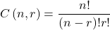
where n is the number of choices (the list of events) and r is how many times you choose or trials. The exclamation point is called the factorial. The factorial instructs you to multiply the number over and over again, “down to one.” For example, if the number is 10, then

In R, just type factorial(10) at the R prompt.
factorial(10)
[1] 3628800
An example
Consider an extrasensory perception, ESP, experiment. We place photocopies of two kinds of cards, “Queen” and “King,” into ten envelopes, one card per envelope (Fig 2). Thus, an envelope either contains a “Queen” or a “King.”

Figure 2. Playing cards with images commemorating 150th anniversary of Charles Darwin’s Origin of Species. (Design John R. C. White, Master of the Worshipful Company of Makers of Playing Cards 2008 to 2009.)
We shuffle the envelopes containing the cards and volunteers guess the contents of the envelopes, one at a time. We score the correct choices after all envelopes had been guessed. (It’s really hard to set these kinds of experiments up to rule out subtle cues and other kinds of experimental error! Diaconis 1978, Pigliucci 2010, pp. 77 – 83.) By chance alone we would expect 50% correct (eg, one way to game the system would have been for the volunteer simply to guess “Queen” every time; since we had placed five “Queen” cards the volunteer would end up being right 50%).
What are the possible combinations?
Let’s start with one correct; the volunteer could be right by guessing the first one correctly, then getting the next nine wrong, or equivalently, the first choice was wrong, but the second was correct followed by eight incorrect choices, and so on.
We need math!
Let n = 10 and r = 1
Using the formula above we have
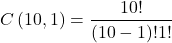
or ten ways to get one out of ten correct. This is the number of combinations without replacement.
In R, we can use the function choose(), included in the base install of R. At the R prompt type
choose(10,1)
and R returns
[1] 10
For permutations, use choose(n,k)*factorial(k).
To get permutations for larger sets, you’ll need to write a function or take advantage of functions written by others and available in packages for R. See gtools package, which contains programming tools for R. There are several packages that can be used to expand capabilities of working with permutations and combinations. For example, install a package and library called combinat and then run the combn() function, together with the dim() function, which will return
dim(combn(10,1))[2]
[1] 10
R explained
In the combn() the “10” is the total number of envelopes and the “1” is how many correct guesses. We also used the dim() function to give us the size of the result. The dim() function returns two numbers, the number of rows and the number of columns — combn() returns a matrix and so dim() saves you the trouble of counting the outcomes — the “[2]” tells R to return the total number of columns in the matrix created by combn(). Here’s the output from combn() , but without the dim() function
combn(10,1)
     [,1] [,2] [,3] [,4] [,5] [,6] [,7] [,8] [,9] [,10]
[1,]    1    2    3    4    5    6    7    8    9    10
in order, we see that there is one case where the success came the first time [1,1], another case where success came on the second try [1,2] and so on.
We can write a simple function to return the combinations
for (many in seq(0, 10, by = 1)){
    print(choose(10, many))
}
an inelegant function, but it works well enough, returning
[1] 1
[1] 10
[1] 45
[1] 120
[1] 210
[1] 252
[1] 210
[1] 120
[1] 45
[1] 10
[1] 1
Note that there’s only one way to get zero correct, only one way to get all ten correct.
For completion, what would be the permutations? Use the permn() function (same combinat library) along with length() function to get the number of permutations
length(permn(10))
[1] 3628800
Continue the example
Back to our ESP problem. If we continue with the formula, how many ways to get two correct? Three correct? And so on, we can show the results in a bar graph (Fig 3).
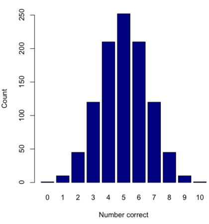
Figure 3. Bar chart of the combinations of correct guesses out of 10 attempts (graph was presented in Chapter 4.1).
The graph in Figure 3 was made in R
Combos <- seq(0,10, by=1)
HowMany <- c(1,10,45,120,210,252,210,120,45,10,1)
barplot(HowMany, names.arg = Combos, xlab = "Number correct", ylab = "Count",col = "darkblue")
If you recall, we had two students score eight out of ten. Is this evidence of “ESP?” It certainly seems pretty good, but how rare is this to score 8 out of 10? The total number of outcomes was

Eight out of ten could be achieved in 45 different ways, so
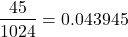
So, eight out of ten is pretty unlikely! Is it evidence for ESP powers in our Biostatistics class? In fact, at the traditional Type I error rate of 5% used in biology and other sciences to evaluate inferences from statistical tests (See Chapter 8), we would say that this observation was statistically significant. Given that this would be an extraordinary claim, this should give you an important clue that statistical significance is not the same thing as evidence for the claim of ESP.
Note 2: This is a good example where frequentist approach may not be the best approach — the Bayesian prior probability for ESP is vanishingly low. See O’Hagan (2006) for a similar ESP problem worked from a Bayesian perspective.
In other words, Is our result biologically significant? Probably not, but I’ll keep my eyes on you, just in case.
Conclusions
Combinations or permutations?
Combinations refers to groups of n things taken k times without repetition. Note that order does not matter, just the combination of things. Permutations, on the other hand, specifically relate the number of ways a particular arrangement can show up.
Questions
- Calculate the combinations, from zero correct to ten correct, from our ESP experiment, ie, confirm the numbers reported in Figure 3.
- Consider our ESP tests based on guessing cards. Let’s say that one subject repeatedly reports correct guesses at a rate greater than expected by chance. Why or why not should we view this as evidence the person may have extrasensory perception?
- Return to our TATA box example. The number of protein-coding genes in the human genome is presently estimated to be 20,620 (NCBI August 2025). Given that each gene has one promoter sequence, what proportion of TATA boxes are not associated with protein-coding genes?
- Assuming a standard 52-card deck, how many possible 5-card poker hands — the set of cards a player holds during a round of play — are there?
Quiz Chapter 6.3
Combinations and permutations
Chapter 6 contents
- Introduction
- Some preliminaries
- Ratios and probabilities
- Combinations and permutations
- Types of probability
- Discrete probability distributions
- Continuous distributions
- Normal distribution and the normal deviate (Z)
- Moments
- Chi-square distribution
- t distribution
- F distribution
- References and suggested readings