20.10 – Growth equations and dose response calculations
Introduction
In biology, growth may refer to increase in cell number, change in size of an individual across development, or increase of number of individuals in a population over time. Nonlinear, time-series, several models proposed to fit growth data, including the Gompertz, logistic, and the von Bertalanffy. These models fit many S-shaped growth curves. These models are special cases of generalized linear models, also called Richard curves.
Growth example
This page describes how to use R to analyze growth curve data sets.
| Hours | Abs |
|---|---|
| 0.000 | 0.002207 |
| 0.274 | 0.010443 |
| 0.384 | 0.033688 |
| 0.658 | 0.063257 |
| 0.986 | 0.111848 |
| 1.260 | 0.249240 |
| 1.479 | 0.416236 |
| 1.699 | 0.515578 |
| 1.973 | 0.572632 |
| 2.137 | 0.589528 |
| 2.466 | 0.619091 |
| 2.795 | 0.608486 |
| 3.123 | 0.621136 |
| 3.671 | 0.616850 |
| 4.110 | 0.614689 |
| 4.548 | 0.614643 |
| 5.151 | 0.612465 |
| 5.534 | 0.606082 |
| 5.863 | 0.603933 |
| 6.521 | 0.595407 |
| 7.068 | 0.589006 |
| 7.671 | 0.578372 |
| 8.164 | 0.567749 |
| 8.877 | 0.559217 |
| 9.644 | 0.546451 |
| 10.466 | 0.537907 |
| 11.233 | 0.537826 |
| 11.890 | 0.529300 |
| 12.493 | 0.516551 |
| 13.205 | 0.505905 |
| 14.082 | 0.491013 |
Key to parameter estimates: y0 is the lag, mumax is the growth rate, and K is the asymptotic stationary growth phase. The spline function does not return an estimate for K.
R code
require(growthrates)
#Enter the data. Replace these example values with your own
#time variable (Hours)
Hours <- c(0.000, 0.274, 0.384, 0.658, 0.986, 1.260, 1.479, 1.699, 1.973, 2.137, 2.466, 2.795, 3.123, 3.671, 4.110, 4.548, 5.151, 5.534, 5.863, 6.521, 7.068, 7.671, 8.164, 8.877, 9.644, 10.466, 11.233, 11.890, 12.493, 13.205, 14.082)
#absorbance or concentration variable (Abs)
Abs <- c(0.002207, 0.010443, 0.033688, 0.063257, 0.111848, 0.249240, 0.416236, 0.515578, 0.572632, 0.589528, 0.619091, 0.608486, 0.621136, 0.616850, 0.614689, 0.614643, 0.612465, 0.606082, 0.603933, 0.595407, 0.589006, 0.578372, 0.567749, 0.559217, 0.546451, 0.537907, 0.537826, 0.529300, 0.516551, 0.505905, 0.491013)
#Make a dataframe and check the data; If error, then check that variables have equal numbers of entries
Yeast <- data.frame(Hours,Abs); Yeast
#Obtain growth parameters from fit of a parametric growth model
#First, try some reasonable starting values
p <- c(y0 = 0.001, mumax = 0.5, K = 0.6)
model.par <- fit_growthmodel(FUN = grow_logistic, p = p, Hours, Abs, method=c("L-BFGS-B"))
summary(model.par)
coef(model.par)
#Obtain growth parameters from fit of a nonparametric smoothing spline
model.npar <- fit_spline(Hours,Abs)
summary(model.npar)
coef(spline.md)
#Make plots
par(mfrow = c(2, 1))
plot(Yeast, ylim=c(0,1), cex=1.5,pch=16, main="Parametric Nonlinear Growth Model", xlab="Hours", ylab="Abs")
lines(model.par, col="blue", lwd=2)
plot(model.npar, ylim=c(0,1), lwd=2, main="Nonparametric Spline Fit", xlab="Hours", ylab="Abs")
Results from example code
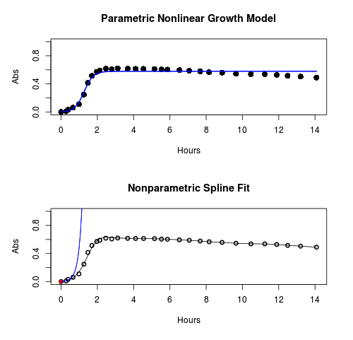
Figure 1. Top: Parametric Nonlinear Growth Model; Bottom: Nonparametric Spline Fit
LD50
In toxicology, the dose of a pathogen, radiation, or toxin required to kill half the members of a tested population of animals or cells is called the lethal dose, 50%, or LD50. This measure is also known as the lethal concentration, LC50, or properly after a specified test duration, the LCt50 indicating the lethal concentration and time of exposure. LD50 figures are frequently used as a general indicator of a substance’s acute toxicity. A lower LD50 is indicative of increased toxicity.
The point at which 50% response of studied organisms to range of doses of a substance (e.g., agonist, antagonist, inhibitor, etc.) to any response, from change in behavior or life history characteristics up to and including death can be described by the methods described in this chapter. The procedures outlined below assume that there is but one inflection point, i.e., an “s-shaped” curve, either up or down; if there are more than one inflection points, then the logistic equations described will not fit the data well and other choices need to be made (see Di Veroli et al 2015). We will use the drc package (Ritz et al 2015).
Example
First we’ll work through use of R. We’ll follow up with how to use Solver in Microsoft Excel.
After starting R, load the drc library.
library(drc)
Consider some hypothetical 24-hour survival data for yeast exposed to salt solutions. Let resp equal the variable for frequency of survival (e.g., calculated from OD660 readings) and NaCl equal the millimolar (mm) salt concentrations or doses.
At the R prompt type
resp <- c(1,1,1,.9,.7,.3,.4,.2,0,0,0)
NaCl=seq(0,1000,100)
#Confirm sequence was correctly created; alternatively, enter the values.
NaCl
[1] 0 100 200 300 400 500 600 700 800 900 1000
#Make a plot
plot(NaCl,resp,pch=19,cex=1.2,col="blue",xlab="NaCl [mm]",ylab="Survival frequency")
And here is the plot (Fig. 2).
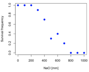
Figure 2. Hypothetical data set, survival of yeast in different salt concentrations.
Note the sigmoidal “S” shape — we’ll need an logistic equation to describe the relationship between survival of yeast and NaCl doses.
The equation for the four parameter logistic curve, also called the Hill-Slope model, is

where c is the parameter for the lower limit of the response, d is the parameter for the upper limit of the response, e is the relative EC50, the dose fitted half-way between the limits c and d, and b is the relative slope around the EC50. The slope, b, is also known as the Hill slope. Because this experiment included a dose of zero, a three parameter logistic curve would be appropriate. The equation simplifies to

EC50 from 4 parameter model
Let’s first make a data frame
dose <- data.frame(NaCl, resp)
Then call up a function, drm, from the drc library and specify the model as the four parameter logistic equation, specified as LL.4(). We follow with a call to the summary command to retrieve output from the drm function. Note that the four-parameter logistic equation
model.dose1 = drm(dose,fct=LL.4())
summary(model.dose1)
And here is the R output.
Model fitted: Log-logistic (ED50 as parameter) (4 parms)
Parameter estimates:
                   Estimate  Std. Error    t-value  p-value
b:(Intercept)      3.753415    1.074050   3.494636   0.0101
c:(Intercept)     -0.084487    0.127962  -0.660251   0.5302
d:(Intercept)      1.017592    0.052460  19.397441   0.0000
e:(Intercept)    492.645128   47.679765  10.332373   0.0000

Residual standard error:
0.0845254 (7 degrees of freedom)
The EC50, technically the LD50 because the data were for survival, is the value of e: 492.65 mM NaCl.
You should always plot the predicted line from your model against the real data and inspect the fit.
At the R prompt type
plot(model.dose1, log="",pch=19,cex=1.2,col="blue",xlab="NaCl [mm]",ylab="Survival frequency")
As long as the plot you made in earlier steps is still available, R will add the line specified in the lines command. Here is the plot with the predicted logistic line displayed (Fig. 3).
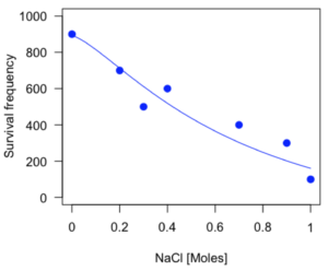
Figure 3. Logistic curve added to Figure 1 plot.
While there are additional steps we can take to decide is the fit of the logistic curve was good to the data, visual inspection suggests that indeed the curve fits the data reasonably well.
More work to do
Because the EC50 calculations are estimates, we should also obtain confidence intervals. The drc library provides a function called ED which will accomplish this. We can also ask what the survival was at 10% and 90% in addition to 50%, along with the confidence intervals for each.
At the R prompt type
ED(model.dose1,c(10,50,90), interval="delta")
And the output is shown below.
Estimated effective doses
(Delta method-based confidence interval(s))
     Estimate Std. Error   Lower   Upper
1:10  274.348     38.291 183.803  364.89
1:50  492.645     47.680 379.900  605.39
1:90  884.642    208.171 392.395 1376.89
Thus, the 95% confidence interval for the EC50 calculated from the four parameter logistic curve was between the lower limit of 379.9 and an upper limit of 605.39 mm NaCl.
EC50 from 3 parameter model
Looking at the summary output from the four parameter logistic function we see that the value for c was -0.085 and p-value was 0.53, which suggests that the lower limit was not statistically different from zero. We would expect this given that the experiment had included a control of zero mm added salt. Thus, we can explore by how much the EC50 estimate changes when the additional parameter c is no longer estimated by calculating a three parameter model with LL.3().
model.dose2 = drm(dose,fct=LL.3())
summary(model.dose2)
R output follows.
Model fitted: Log-logistic (ED50 as parameter) with lower limit at 0 (3 parms)
Parameter estimates:
               Estimate Std. Error   t-value p-value
b:(Intercept)   4.46194    0.76880   5.80378   4e-04
d:(Intercept)   1.00982    0.04866  20.75272   0e+00
e:(Intercept) 467.87842   25.24633  18.53253   0e+00
Residual standard error:
 0.08267671 (8 degrees of freedom)
The EC50 is the value of e: 467.88 mM NaCl.
How do the four and three parameter models compare? We can rephrase this as as statistical test of fit; which model fits the data better, a three parameter or a four parameter model?
At the R prompt type
anova(model.dose1, model.dose2)
The R output follows.
1st mode
fct:      LL.3()
2nd model
fct:      LL.4()
ANOVA table
          ModelDf      RSS Df F value p value
2nd model       8 0.054684
1st model       7 0.050012  1  0.6539  0.4453
Because the p-value is much greater than 5% we may conclude that the fit of the four parameter model was not significantly better than the fit of the three parameter model. Thus, based on our criteria we established in discussions of model fit in Chapter 16 – 18, we would conclude that the three parameter model is the preferred model.
The plot below now includes the fit of the four parameter model (red line) and the three parameter model (green line) to the data (Fig. 4).
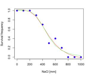
Figure 4. Four parameter (red) and three parameter (green) logistic models fitted to data.
The R command to make this addition to our active plot was
lines(dose,predict(model.dose2, data.frame(x=dose)),col="green")
We continue with our analysis of the three parameter model and produce the confidence intervals for the EC50 (modify the ED() statement above for model.dose2 in place of model.dose1).
Estimated effective doses
(Delta method-based confidence interval(s))
     Estimate Std. Error   Lower  Upper
1:10  285.937     33.154 209.483 362.39
1:50  467.878     25.246 409.660 526.10
1:90  765.589     63.026 620.251 910.93
Thus, the 95% confidence interval for the EC50 calculated from the three parameter logistic curve was between the lower limit of 409.7 and an upper limit of 526.1 mm NaCl. The difference between upper and lower limits was 116.4 mm NaCl, a smaller difference than the interval calculated for the 95% confidence intervals from the four parameter model (225.5 mm NaCl). This demonstrates the estimation trade-off: more parameters to estimate reduces the confidence in any one parameter estimate.
Additional notes of EC50 calculations
Care must be taken that the model fits the data well. What if we did not have observations throughout the range of the sigmoidal shape? We can explore this by taking a subset of the data.
dd = dose[1:6,]
Here, all values after dose 500 were dropped
dd
  resp dose
1  1.0    0
2  1.0  100
3  1.0  200
4  0.9  300
5  0.7  400
6  0.3  500
and the plot does not show an obvious sigmoidal shape (Fig. 5).
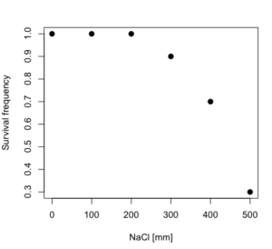
Figure 5. Plot of reduced data set.
We run the three parameter model again, this time on the subset of the data.
model.dosedd = drm(dd,fct=LL.3())
summary(model.dosedd)
Output from the results are
Model fitted: Log-logistic (ED50 as parameter) with lower limit at 0 (3 parms)
Parameter estimates:
                Estimate Std. Error    t-value p-value
b:(Intercept)   6.989842   0.760112   9.195801  0.0027
d:(Intercept)   0.993391   0.014793  67.153883  0.0000
e:(Intercept) 446.882542   5.905728  75.669344  0.0000
Residual standard error:
 0.02574154 (3 degrees of freedom)
Conclusion? The estimate is different, but only just so, 447 vs. 468 mm NaCl.
Thus, within reason, the drc function performs well for the calculation of EC50. Not all tools available to the student will do as well.
NLopt and nloptr
draft
Free open source library for nonlinear optimization.
Steven G. Johnson, The NLopt nonlinear-optimization package, http://github.com/stevengj/nlopt
https://cran.r-project.org/web/packages/nloptr/vignettes/nloptr.html
Alternatives to R
What about online tools? There are several online sites that will allow students to perform these kinds of calculations. Students familiar with MatLab know that it can be used to solve nonlinear equation problems. An open source alternative to MatLab is called GNU Octave, which can be installed on a personal computer or run online at http://octave-online.net. Students also may be aware of other sites, e.g., mycurvefit.com and IC50.tk.
Both of these free services performed well on the full dataset (results not shown), but fared poorly on the reduced subset: mycurvefit returned a value of 747.64 and IC50.tk returned an EC50 estimate of 103.6 (Michael Dohm, pers. obs.).
Simple inspection of the plotted values shows that these values are unreasonable.
EC50 calculations with Microsoft Excel
Most versions of Microsoft Excel include an add-in called Solver, which will permit mathematical modeling. The add-in is not installed as part of the default installation, but can be installed via the Options tab in the File menu for a local installation or via Insert for the Microsoft Office online version of Excel (you need a free Microsoft account). The following instructions are for a local installation of Microsoft Office 365 and were modified from information provided by sharpstatistics.co.uk.
After opening Excel, set up worksheet as follows. Note that in order to use my formulas your spreadsheet values need to be set up exactly as I describe.
- Dose values in column A, beginning with row 2
- Response values in column B, beginning with row 2
- In column F type
bin row 2,cin row 3,din row 4, andein row 5. - In cells G2 – G5, enter the starting values. For this example, I used b = 1, c = 0, d = 1, e = 400.
- For your own data you will have to explore use of different starting values.
- Enter headers in row 1.
- Column A
Dose - Column B
Response - Column C
Predicted - Column D
Squared difference - Column F
Constants
- Column A
- In cell C14 enter
sum squares - In cell D14 enter
=sum(D2:D12)
Here is an image of the worksheet (Fig. 6), with equations entered and values updated, but before Solver run.
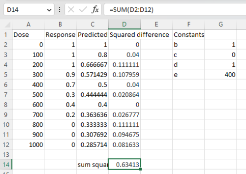
Figure 6. Screenshot Microsoft Excel worksheet containing our data set (col A & B), with formulas added and calculated. Starting values for constants in column G, rows 2 – 4.
Next, enter the functions.
- In cell C2 enter the four parameter logistic formula — type everything between the double quotes: “
=$G$3+(($G$4-$G$3)/(1+(A2/$G$5)^$G$2))“. Next, copy or drag the formula to cell C12 to complete the predictions.- Note: for a three parameter model, replace the above formula with “
=(($G$4)/(1+(A2/$G$5)^$G$2))“.
- Note: for a three parameter model, replace the above formula with “
- In cell D2 type everything between the double quotes: “
=(B2-C2)^2“. - Next, copy or drag the formula to cell
D12to complete the predictions. - Now you are ready to run solver to estimate the values for b, c, d, and e.
- Reminder: starting values must be in cells
G2:G5
- Reminder: starting values must be in cells
- Select cell
D14and start solver by clicking on Data and looking to the right in the ribbon.
Solver is not normally installed as part of the default installation of Microsoft Excel 365. If the add-in has been installed you will see Solver in the Analyze box (Fig. 7).
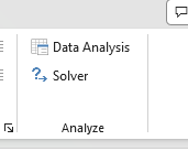
Figure 7. Screenshot Microsoft Excel, Solver add-in available.
If Solver is not installed, go to File → Options → Add-ins (Fig. 8).
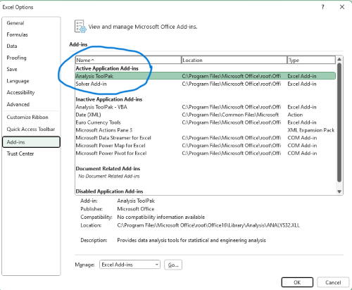
Figure 8. Screenshot Microsoft Excel, Solver add-in available and ready for use.
Go to Microsoft support for assistance with add-ins.
With the spreadsheet completed and Solver available, click on Solver in the ribbon (Fig. 7) to begin. The screen shot from the first screen of Solver is shown below (Fig. 9).
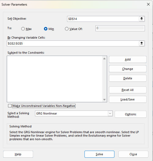
Figure 9. Screenshot Microsoft Excel solver menu.
Setup Solver
- Set Objective, enter the absolute cell reference to the sum squares value, \
$D$14 - Set To: Min.
- For By Changing Variable Cells, enter the range of cells for the four parameters, $G$2:$G$5
- Uncheck the box by “Make Unconstrained Variables Non-Negative.”
- Where constraints refers to any system of equalities or inequalities equations imposed on the algorithm.
- Select a Solving method, choose “GRG Nonlinear,” the nonlinear programming solver option (not shown in Fig. 7, select by clicking on the down arrow).
- Click Solve button to proceed.
GRG Nonlinear is one of many optimization methods. In this case we calculate the minimum of the sum of squares — the difference between observed and predicted values from the logistic equation — given the range of observed values. GRG stands for Generalized Reduced Gradient and finds the local optima — in this case the minimum or valley — without any imposed constraints. See solver.com for additional discussion of this algorithm.
If all goes well, this next screen (Fig. 10) will appear which shows the message, “Solver has converged to the current solution. All constraints are satisfied.”
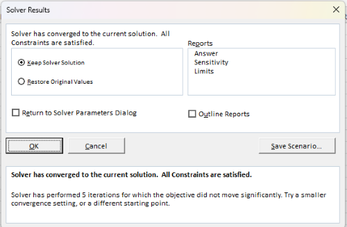
Figure 10. Screenshot solver completed run.
Click OK and note that the values of the parameters have been updated (Table 1).
Table 1. Four parameter logistic model, results from Solver
| Constant | Starting values | Values after solver |
| b | 1 | 3.723008382 |
| c | 0 | -0.088865487 |
| d | 1 | 1.017964505 |
| e | 400 | 493.9703594 |
Note the values obtained by Solver are virtually identical to the values obtained in the drc R package. The differences are probably because of the solver algorithm.
More interestingly, how did Solver do on the subset data set? Here are the results from a three parameter logistic model (Table 2).
Table 2. Three parameter logistic model, results from Solver
| Constant | Starting values | Full dataset, Solver results |
Subset, Solver results |
| b | 1 | 3.723008382 | 6.989855948 |
| d | 1 | 1.017964505 | 0.993391264 |
| e | 400 | 493.9703594 | 446.8819282 |
The results are again very close to results from the drc R package.
Thus, we would conclude that Solver and Microsoft Excel would be a reasonable choice for EC50 calculations, and much better than IC50.tk and mycurvefit.com. The advantages of R over Microsoft Excel is that the model building is more straightforward than entering formulas in the cell reference format required by Excel.
Questions
[pending]
References and suggested readings
Beck B, Chen YF, Dere W, et al. Assay Operations for SAR Support. 2012 May 1 [Updated 2012 Oct 1]. In: Sittampalam GS, Coussens NP, Nelson H, et al., editors. Assay Guidance Manual [Internet]. Bethesda (MD): Eli Lilly & Company and the National Center for Advancing Translational Sciences; 2004-. Available from: www.ncbi.nlm.nih.gov/books/NBK91994/
Di Veroli G. Y., Fornari C., Goldlust I., Mills G., Koh S. B., Bramhall J. L., Richards, F. M., Jodrell D. I. (2015) An automated fitting procedure and software for dose-response curves with multiphasic features. Scientific Reports 5: 14701.
Ritz, C., Baty, F., Streibig, J. C., Gerhard, D. (2015) Dose-Response Analysis Using R PLOS ONE, 10(12), e0146021
Tjørve, K. M., & Tjørve, E. (2017). The use of Gompertz models in growth analyses, and new Gompertz-model approach: An addition to the Unified-Richards family. PloS one, 12(6), e0178691.
Chapter 20 contents
- Additional topics
- Area under the curve
- Peak detection
- Baseline correction
- Surveys
- Time series
- Dimensional analysis
- Estimating population size
- Diversity indexes
- Survival analysis
- Growth equations and dose response calculations
- Plot a Newick tree
- Phylogenetically independent contrasts
- How to get the distances from a distance tree
- Binary classification
- Meta-analysis
/MD
2.4 – Experimental Design and rise of statistics in medical research
Experiments and observations: Finding answers.
.
How to identify cause and effect, and the kinds of evidence that can be inferred from the various approaches to study causes of disease has became a major source of disagreement in the news. In a fascinating study, Pew Research Center reported “half of U.S. adults under 50 say they get health and wellness information from social media influencers or podcasts,” and, only about 17% of these influencers report “conventional medicine” training (Report, May 7 2026). For our purposes, I made substantial updates to this page in the fifth month after WHO had declared the Covid-19 pandemic (CDC timeline), and continue to do so today.
The pandemic left many life-lessons, for scientists and public-health supporters, but also for everyone who lived through those times. One of the lessons was how to deal with the challenges of finding treatments in real time. If you followed the news early in the pandemic, you know of the appeal from some (including Donald Trump, the then-President of the United States, Boseley 2020), for use of an anti-parasite drug, hydroxychloroquine, as prophylactic or treatment for active Covid-19 infection (cf. Liu et al 2020). The FDA as well as other institutions rapidly advised against use, in part because experimental design concerns were raised for early studies (Kupferschmidt, 2020). The issue remains contentious for some (eg, Health and Human Services Secretary Robert F. Kennedy Jr., CNN August 2, 2026 interview).
Thus, job number one for students of biostatistics is to learn how to weigh arguments for or against therapies or treatments offered. The purpose of this page is to introduce these issues — how to judge whether a treatment is effective or not.
We will spend some time later on statistical aspects of experimental design (Chapter 5), but we begin with Randomized Control Trials, or RCT, as a model for our discussion of experimental studies. The RCT we recognize today owes its beginning to the 1948 studies on streptomycin use to treat tuberculosis (British Medical Research Council 1948), but of course, the foundations of RCT and experimental design in general, go back much earlier than that date (Chalmers 2011, Hairton and Locascio 2018). For a number of reasons the RCT — experimental, prospective, double-blind clinical trial with random selection of subjects from a reference population and random assignment of subjects to a treatment group or an appropriate placebo treatment control group — is considered the “gold standard” method for producing knowledge (Kaptchuk 2001, Hairton and Locascio 2018).
Note 1. I use the phrase “gold standard” associated with the RCT in the historical context intended by the authors cited. Unfortunately, in 2025, the phrase “gold standard science” has become political (Lewandowsky 2025, Mervis 2025). What we can agree on is characteristics of research as good science: “reproducible; transparent; communicative of error and uncertainty; collaborative and interdisciplinary; skeptical of its findings and assumptions; structured for falsifiability of hypotheses; subject to unbiased peer review; accepting of negative results as positive outcomes; and without conflicts of interest,” Sec. 3. Restoring Gold Standard Science, Presidential Executive Order, May 23, 2025. But even this list is not above scrutiny.
This discourse is way above my pay grade, but for starters, I would replace “without conflicts of interest” with “without disclosure of potential conflicts of interest.” The latter is practical, the former is likely not at all achievable. After all, even where a conflict exists, it does not immediately follow that the reported science is bad, that the conflict is evidence by itself of bias. Reporting conflicts warns the reader that results and conclusions may warrant further scrutiny, but outright dismissal is itself contrary to good science practice. Certainly, there are other aspects to defining what is and what is not good science. And, “gold standard” is just a metaphor (Love 2003), and, frankly, a very out-dated one. The United States and most other nations long ago gave up — for many good reasons — the gold standard as a monetary standard.
Technically, RCT are intervention trials, a specific application of the more general definition of an experiment. That is, the researchers tests a potential drug or therapy in people to observe its effect while holding other variables constant. Experimental studies imply that the researcher imposed treatments or controls onto subjects. The subjects are followed and outcomes are recorded. Thus, experiments by definition are also prospective studies — the outcome is recorded for subjects after some period of time. With a well-designed experiment, the researcher may have evidence to support the claim that, for example, Treatment A causes the outcome.
RCT applied to human health can have profound impact on lives.
The ALLHAT-LLT (JAMA, 2002) trial tested whether adding the cholesterol-lowering drug pravastatin to standard care would reduce heart attacks and deaths in people with high blood pressure and moderately high cholesterol. The study found no significant benefit compared to usual care, suggesting that statin therapy may not always provide extra protection in this group. Its results helped refine how doctors balance blood pressure and cholesterol treatment in heart disease prevention.
The Women’s Health Initiative (JAMA, 2002) trial tested the effects of combined estrogen and progestin therapy in healthy postmenopausal women. It found that while the therapy slightly reduced the risk of fractures and colon cancer, it increased the risk of heart disease, stroke, and breast cancer. These results transformed medical guidance by showing that hormone therapy should not be routinely used to prevent chronic disease in postmenopausal women.
The Du Toit et al. (NEJM, 2015) study showed that introducing peanut-containing foods early in life — rather than avoiding them — greatly reduced the risk of developing peanut allergies in high-risk infants. This landmark randomized trial changed how doctors think about food allergies, leading to new guidelines that encourage early introduction instead of avoidance.
And more recently, we have study reported by Deanfield et al (Lancet, 2025), which found that semaglutide reduced the risk of major adverse cardiovascular events (MACE) in adults with overweight or obesity and established cardiovascular disease—even if they did not lose much weight or had lower baseline adiposity.
In contrast, observational studies are those in which treatments arise by acts of nature. In both experiments and observational studies, there can be treatment and control groups; the distinction between the types of studies is how assignment of subjects to treatments were affected. Observational studies generally are retrospective studies — the outcome has already occurred, the researcher follows up to identify differences among the groups that may account for different outcomes. Examples of observational, retrospective study designs include cross-sectional and case control; cohort studies are prospective studies. Observational studies are discussed further in Chapter 5.4 – Clinical trials.
Compared to observational studies, in principle, experiments can establish cause and effect. Cause and effect refers to an explanation about relationship between two events or objects. In biology, Ernst Mayr (1904 – 2005) distinguished between two levels of explanation, proximate (how) explanations and ultimate (why) explanations (Mayr 1961, cf. Laland et al. 2011). As you know, our mechanism for identifying cause and effect is application of the Scientific Method (Chapter 2.5). Discussions of how to detect cause and effect are provided throughout this book, but emphasized in a few sections (Chapter 16.2 and 16.3).
Good experiments.
The principles of good experiments include many steps beyond simply choosing treatments and controls. In Chapter 5 we’ll go into more depth, but I wished to list for you some of the key principles of good experimental design. With respect to human-subject research, the researcher needs to protect against many sources of potential bias.
- Randomization of subjects assigned to treatment groups controls for individual differences.
- Controls (eg, Placebos) are a means to establish controls in a study so that effects may be attributed to the active treatment.
- Single-blind implies that the subject does not know what treatment was given.
- Double-blind implies that not only is the subject unaware of the treatment received, but, crucially, neither does the researcher.
- The double-blind design — neither the patient-subject nor the researchers know who received the placebo or the treatment — controls for subtle biases.
Note 2. Experimental control implies researcher imposes conditions to remove possibly confounding effects on the dependent variable — outcome of the experiment. Placebo, derived from Latin placere, to please (but see Aronson 1999). Placebo refers to an inert substance (“sugar pill”), or to a substance with known activity but without effect on the target condition or “wrong indication” (eg, antibiotics administered for viral infection), given to research subjects in lieu of the active treatment of interest (the hypothesis). Thus, placebos are examples of treatment controls.
The placebo effect is improvement of subjects who received the placebo and not active treatment (Pardo-Cabello et al 2022). In contrast, nocebo effects are adverse effects attributed to placebo treatment. Under most circumstances, placebo applies to humans only because placebo effects are thought to be product of psychological factors, although mechanisms of action are in dispute. Is sentience necessary for a placebo effect (cf. McMillan 1999)?
The experimenter may influence the outcome of the experiment if knowledge about who received the placebo or the new drug; the subject may respond differently with knowledge that they received the placebo and not the new drug. The key intent in this experimental design is to avoid systematic error, errors in studies that may occur because of our conscious and unconscious beliefs and biases. Placebos are used as treatments because people (and animals!) sometimes get better (or worse) with or without treatment; thus, to be effective, subjects receiving a new drug must get better more frequently than do subjects on placebo. Importantly, the well-designed placebo allows the researcher to gain insight into the mechanism of action by the new drug.
A case to consider: Comparing migraine treatments.
.
Consider the following experiment (Diener et al 2006; see also Liu et al 2018): subjects who had several migraines per month were treated with acupuncture, sham-acupuncture, or standard treatments including beta blockers, calcium channel blockers, or antiepileptic drugs. After 26 weeks the reductions in reported migraines was compared. The authors reported that there was no difference in numbers of migraines among patients who received the different therapy treatments. The authors conclude that because acupuncture lacks side-effects that may occur with standard therapies acupuncture may be a good choice for patients seeking relief from migraine. This is a classic experiment — subjects were assigned to treatments by the researchers. At least in principle, if one treatment group showed better outcomes, the improvement could be attributed to the treatment.
Another case to consider: When the cause isn’t clear.
.
Consider the following example. My dad was diagnosed with lung cancer in his late 70s; his left lung showed many spots when imaged and biopsy confirmed. Surgeons removed half of the lung and after several years he was considered cancer free. Why did he develop cancer in the first place? If you immediately think, “He’s a smoker,” that’s not a good explanation — and shame on you, you’re first instinct was to blame the patient (see discussion in Huff 2013). Dad last smoked tobacco in his early thirties (latency smoking-lung cancer link about 20 years, Lipfert et al 2019).
Tobacco smoking is not the only environmental trigger for lung cancer. Cancer of the lung in non-smokers is the seventh leading cause of cancer mortality worldwide (Field and Withers 2012). Long term exposure to radon gas, a naturally occurring, radioactive noble gas has been linked to lung cancer (EPA). I grew up on Vashon Island, Washington, in a non-smoking home environment. Radon levels on Vashon Island and other areas around Puget Sound are low (source: Washington State Department of Health). Radon is out as an explanation.
What other environmental sources may be linked to cancer? Vashon Island is rural, but, as it turned out, within range of effluent from a copper smelter located in nearby Ruston, Pierce County (Fig 1; my home was 17 km distance from the smelter).

Figure 1. Left: ASARCO smelter, Ruston, Washington, image from Department of Ecology, State of Washington. Direction of smoke from the stack is north, toward Vashon Island. Right: Voronoi map of arsenic and lead affected areas. image from kingcounty.gov. Darker regions correspond to heavier arsenic and lead contamination of soils.
The smelter was last in operation in 1986 and was torn down in 1993 (EPA publication number 910R94001). The smelter stack rose more than 500 feet dispersing smoke laden with heavy metals, notably inorganic arsenic and lead, into the air (Bromenshenk et al. 1985). Over the smelter’s 68 years of service, winds carried away the smoke to my island and to other areas known now as the “Ruston-Vashon Island Exposure Pathway” (Kalman et al 1990). The former smelter site was among the first listed Superfund sites (1983) in the United States by the EPA. Thus, tens of thousands of people were (and continue to be) exposed to the heavy metals deposited into the soils, forming a distinct exposure group (Milham & Strong 1974; Kalman et al 1990; EPA 2000). Arsenic exposure can be via inhalation, skin, or in drinking water — areas of Vashon-Maury island continue to have high levels of arsenic in both the soil and in any domestic water wells (PublicationNo. 14-09-044, Department of Ecology State of Washington).
Note 3: A personal comment — I stumbled onto the article by Bromenshenk and colleagues by accident. Instead of attending lecture, as I often did at the time, I was looking through journals in the research library. I was shocked at this article, because for the first time, I connected the smelter to the island I grew up on. The contamination on the island just wasn’t a conversation.
Is arsenic exposure by inhalation a plausible mechanism for my Dad’s lung cancer? As shown in Fig 1, the soils on Vashon near my home were heavily impacted by the smelter. Exposure could have come about from exposure during routine yard work — I have memories of clouds of dust kicked up by the lawn mower during spring and summers. Thus, an exposure route is possible. What evidence can we come up with?
Figure 2A shows negative association between lung and bronchial cancer incidence rates per 100L persons, adjusted for age, for several Washington state counties between 2000 and 2020 and distance from the smelter in Ruston. For comparison, Figure 2B shows no association between bladder cancer incidence rates per 100K for the same counties and time period and distance from the smelter. Workers exposed to arsenic have higher rates of lung cancer (Sullivan 2007, Wei et al 2019; see Enterline et al 1987 for a study a study based on cancer of workers at the smelter). Cultured lung cells exposed to arsenic associated with changes in gene expression (Clancy et al 2012). Coincidently, two of the family dogs developed and died of cancer as did one female goat. Perhaps my dad’s lung cancer was attributed to long exposure to arsenic (a decade after the cancer, and long after he stopped with yard work, his blood readings for arsenic were in the range of a modest 11 μg/L).
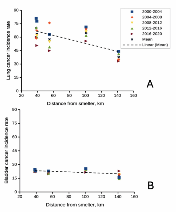
Figure 2. County cancer rates (A, lung and bronchial; B, bladder) from 2000 – 2020 vs distance in kilometers from ASARCO smelter, Ruston, WA. Data compiled from Washington Tracking Network (WTN). The counties were King (55 km), Kitsap (39.28 km), Pierce (38.48 km), San Juan ( 141.43 km), Snohomish (100.73 km), and Spokane (385.34 km).
If this scenario seems plausible, I hope you immediately recognize it as a case of confirmation bias (see Chapter 2.6). Putting aside for a moment the different arsenic species, each with different LD50 (the lethal dose needed to kill half the population — see Chapter 20.10), the difficulty ascribing arsenic as a causal agent for my Dad’s cancer is that many other exposures happened simultaneously. For example, indoor carpets are a primary source of several volatile organic compounds (Haines et al 2020). Prior to 1980 carpets may have included formaldehyde and other known carcinogenic agents. Dad commuted by car between work and home — with a ferry ride between — for decades (until the early 1990s), routinely traveling heavily congested roadways, this during the years prior to and the early years of the Clean Air Act of Environmental Protection Agency of the United States (it wasn’t until 1981 that new cars met EPA emission standards: Clean Air Act timeline here). Thus, all commuters including my Dad were exposed to gasoline combustion emissions, many known to be carcinogenic (Parent et al 2007). Moreover, a limited study by Public Health of Seattle and King County (2001) found rates of cancer on Vashon between 1980 and 1988 were similar to other areas in King County.
Summary.
It’s easy to fall into the trap that experiments — and by extension meta-analysis and systematic reviews — are the best tools offered by science for developing knowledge about the world, and other approaches suffer by comparison. But after even a bit of reflection, we should recognize that it can’t be that simple. While we now “know” tobacco cigarette smoking increases lung cancer risk, and many experiments with animal models convincingly show the link (eg, Hutt et al 2005), no human experiment in the strict sense, ie, prospective, randomized control trial, has ever been conducted (hint: it would be unethical, see discussion in Allmark and Tod 2016). Instead, the accumulated evidence from observational studies on exposures of different populations over the years overwhelmingly points to smoking as a leading risk factor (cause) of lung and other cancers — an example of Hill’s guidelines of causality. We end with a quote:
RCTs can play a role in building scientific knowledge and useful predictions but they can only do so as part of a cumulative program, combining with other methods, including conceptual and theoretical development, to discover not ‘what works’, but ‘why things work’ (p 2, Deaton and Cartwright 2017).
Questions.
.
- Write up three learning outcomes for this page. Hint: Point your favorite generative AI to this page and ask for help.
- Was my Dad’s lung cancer attributable to his 40 years plus exposure to soil arsenic (he’s a non-smoker)? How should we approach this question?
- In Diener et al (2006), the authors concluded that because acupuncture lacks side-effects that may occur with standard therapies acupuncture may be a good choice for patients seeking relief from migraine. Do you agree with the authors?
- Ethical standards evolve with time. An ongoing debate in research is whether and how placebos are to be used in human subjects research. Placebos are a means to establish controls in a study so that effects may be attributed to the active treatment. The “gold standard” of clinical trials is considered to be the randomized double-blind design — neither the patient-subject nor the researchers know who receives the placebo or the treatment. Following review of the WHO report on Use of Placebos in Vaccine Trials, pick one study and evaluate whether or not the decision to use placebos was warranted in your opinion.
- I searched PUBMED for “double-blind” by decade and found the following results (August 2018) (Table 1). Open R and/or R Commander and create two variables, then generate a scatter plot. Describe the shape of the relationship between number of publications citing “double-blind” and time (eg, 1950 – 1959, 1960 – 1969, and so on).
| Decade | Publications |
|---|---|
| 1950 | 60 |
| 1960 | 995 |
| 1970 | 7184 |
| 1980 | 24737 |
| 1990 | 39643 |
| 2000 | 53965 |
| 2010 | 69265 |
- Here’s one way to enter this data into R. At the R prompt (or in the R Script window of R Commander), create two variables,
DecadeandPubsDecade <- c(seq(1950, 2020, by=10))Pubs <- c(59,995,7161,24728,39670,54011,57043)Make an XY scatter plotplot(Decade,Pubs) - Repeat the PUBMED search as above but search for “placebo”. Make a table like the one above and provide a scatterplot of your results.
- Is the concept of a placebo relevant if the subjects in your experiment are yeast cells, not humans?
- Similarly, if your subjects are yeast cells, how does the concept of performing experiments “blind” apply?
- Ethical standards change with time. An ongoing debate in research is whether and how placebos are to be used in human subjects research.
- If placebos are so important, why is their use a concern in clinical trials?
- Following review of the WHO report on Use of Placebos in Vaccine Trials (see Readings below), pick one study and evaluate whether or not the decision to use placebos was warranted in your opinion.
R notes for question 5:
<-is an assignment operator (assignOP); everything to the right of<-is assigned to the object named to the left of the<-operator. You can instead use=in place of<-, but because=is also used in other contexts besides assignment, a quick look at blogs by data scientists will find a preference to use<-for clarity and consistency.c()“combines” arguments into a vector.seq()is used to generate a sequence of numbers between a lower and an upper limit; ifby = nis included, the sequence will be increased by the value n. If omitted, then the sequence is increased by 1.
Quiz Chapter 2.4
Chapter 2 contents.
.
- Introduction
- Why biostatistics?
- Why do we use R Software?
- A brief history of (bio)statistics
- Experimental Design and rise of statistics in medical research
- Scientific method and where statistics fits
- Statistical reasoning
- Chapter 2 – References and suggested reading