16.5 – Instrument reliability and validity

Introduction
Types of reliability
Split-half reliability
Reliability estimators
Questions
Quiz
Chapter 16 contents

Introduction

What’s in a measure? We’ve talked about measurement extensively, eg, Chapter 3.3 . As review, a measure is simply the result of some process used to quantify an object or item of interest. Instead of a number, a measure may return a classification: for a given sample unit, the unit may be categorized as meeting the definition and therefore given a “yes” or it does not (“no”), a dichotomous response. The method used to obtain the measurement is called the instrument. An instrument may indeed be an instrument like a sphygmomanometer or a thermocycler equipped with fluorescent optics. Instrument in this context however also includes questionnaires or surveys intended.

In biology and biomedical research, there are thousands of kinds of measurements one has to choose among depending on the question at hand. In many cases choices are straightforward: in morphometrics, the instruments of choice will be lengths and areas and shapes quantified by rulers and application of well-defined geometry equations. Where multiple measurement approaches apply, reliability analysis can help decide which method to use, or, importantly, whether the different approaches agree. For example, Kruse et al (2017) compared ultra sound and magnetic resonance imaging measurements of Achilles tendon cross-sectional area; they found that although both methods were internally consistent, the methods consistently yielded different results.

In other arenas, the choice of instrument will be less clear. For example, doctors use a questionnaire to rank cardiac patients for attention in perioperative care, the care a surgical patient receives from admittance to release from the hospital, to improve patient outcomes. The questionnaire will include a number of questions intended to provide a summary picture of each patient so that if resources are limited, the most at risk patients may get priority. To the extent the questionnaire in fact is a useful discriminant, then the instrument may benefit both hospital and patients.

In conducting measures one selects instruments that provide valid results. That is, provided the instruments are maintained and well-calibrated, use of a sphygmomanometer by a trained technician will return accurate and valid measures of a subject’s blood pressure. Survey questions also can be evaluated for validity although the extent to which survey questions measure what is intended may be more complex. For example, if the intent is to ascertain a subject’s chance (ie, risk) of graduating from college in the next year, how useful would the following question be if administered to a room filled with first-year students?

Survey question: How old are you now?

Simple enough question, but immediately, several questions come to mind. Do we want our responses in years, months, days, hours, minutes, or seconds? What about for those individuals that know only approximately when they were born, ie, in many parts of the world, registration of birth is irregular. So, we may even wonder about how necessary it is we ask this question of college students in the first place, eg, do we really want to trigger our subjects for a case in which most of our subjects are about the same age?

Perhaps we decide this is important information to ask. When do you start counting? Most Western cultures start the clock at zero when the baby is born. In China and many other Eastern Asian countries, people are born at one. In India, once a person reaches a year plus six months, the person would be considered two years old, whereas in the USA, the person would still be considered one until the second birthday. Thus, depending on the person’s culture identity, responses to this simple question may differ by as much as a year.

Types of reliability

Regardless of instrument, all measures contain error. Hence, even a valid instrument may not return an accurate measure for each subject. The concept of instrument reliability is concerned with error of measurement. Reliability may be defined in at least four contexts:

internal consistency
inter-rater (also called inter-observer reliability)
parallel-forms
test-retest

For an instrument to show internal consistency, this implies that the survey has multiple questions that pertain to the same concept or topic, but written in different ways to reveal effects of word choice, for example. Inter-rater reliability refers to an instrument that when used by different observers (eg, science fair judges), the observers give the same or at least consistent scores for the same test. Parallel forms reliability implies that two surveys on, perhaps scientific literacy in high school students, yield the same conclusions even though each survey has different questions. Test-retest reliability is a straight-forward concept — if the instrument is repeated, are the same scores achieved?

Split-half reliability

Split-half reliability is a method for assessing a measurement tool’s internal consistency by determining if different parts of it produce consistent results. This is done by splitting a single measure (eg, a test or a set of behavioral observations) into two comparable halves, calculating a score for each half, and then finding the correlation between the two sets of scores. For example, the ManyDogs research consortium used split-half design to investigate whether or not dogs consistently interpret human pointing instructions (Espinoza et al 2023). Alternatives to split-half reliability include test-retest reliability, parallel-forms reliability, and inter-rater reliability — see Chapter 12.3, Chapter 14.3 — (Cook and Beckman 2006). These methods assess different aspects of consistency, such as stability over time (test-retest), consistency between two different but equivalent tests (parallel-forms), or agreement between observers (inter-rater). Both ICC and split-half reliability address consistency. The primary distinction is that split-half reliability is a method for assessing the internal consistency of a single test administration, while the Intraclass Correlation Coefficient (ICC) is a more flexible statistical measure used to assess absolute agreement or consistency across different measures, time points, or, most commonly, between multiple raters.

For split-half reliability, a product moment correlation is first calculated between the score of the two halves. A high correlation indicates that all items or observations within the measure are likely assessing the same underlying construct, while a low correlation suggests inconsistency. The correlation coefficient is typically adjusted using the Spearman-Brown prediction formula to estimate the reliability of the original full-length measure.

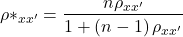
$\begin{align*} \rho*_{xx'}=\frac{n\rho_{xx'}}{1+\left ( n-1 \right )\rho_{xx'}} \end{align*}$

Equation of the Spearman-Brown prediction (or prophecy) formula.

Reliability estimators

In general, correlation-type measures can be used to quantify the extent of reliability (also termed reproducibility or repeatability). The product moment correlation is used to quantify the relationship between two measures where there is clear distinction between the two variables. For example, to quantify the association between body weight and height, the proper correlation to calculate would be the product moment correlation because it is clear that a measure of weight goes with the variable weight whereas height measures goes with the variable height.

But it is less clear which variable should go first in the calculation when you have repeat measures of essentially the same thing. Which goes first, the first observation of sprint running speed over a 100 meters of the second measure of the same person’s performance? Logically, we may say take the first as the X variable and the second as the Y variable, but there is no mathematical justification.

For a more challenging example, consider measures of body mass on male and female birds that are mated, and the researcher wants to assess whether there is a correlation between male and female weight — which variable goes first in the analysis, male weight or female weight? In such cases the intraclass correlation coefficient may be used (Chapter 12.3, Chapter 16.4). The intraclass correlation can be estimated as the ratio of the variance of interest over the sum of the variance of interest plus the variance error. Interest in the case of sprint running would be the two (or more) trials or for the bird weights the variable of interest is weights of male and female birds within a mated pair. The formula for ICC in this context is given by

$\begin{align*} \rho = \frac{\sigma_{B}^2}{\sigma_{B}^2 + \sigma_{e}^2} = \frac{MS_{B} - MS_{e}}{MS_{B} + \left (k - 1 \right ) MS_{e}} \end{align*}$

where k is the number of repeat measures and MS refers to the mean squares from the one-way ANOVA and B and e refer to between (among) subjects and e is the error or within subjects variability.

Cronbach’s alpha is a reliability measure that quantifies the internal consistency of items in a survey or instrument by calculating the average among these items. Cronbach’s alpha will tend to increase as the intercorrelations among test items increase, and in this sense can be taken as an internal consistency estimate of the reliability of test scores.

$\begin{align*} Chronbach's \ \alpha = \frac{k}{k - 1}1 - \frac{\sum_{i = 2}^{n} s_{i}^2 }{s_{T}^2} \end{align*}$

where k is the number of items, s_i² is the variance of the i-th item, and s_T² is the variance of the total score after summing all items.

Cronbach’s alpha is one of the oldest measures, and at least in part because of how long ago it was introduced, is very common as a measure of reliability. However, there are other estimators and in some aspects these perform better than Cronbach’s alpha.

Reliability statistics like Cronbach’s alpha are available in the R package psych. See also R package agRee.

Example. Judging of posters

library(psych)
alpha(myJudge)

Output from R

Reliability analysis 
Call: alpha(x = myJudge)

raw_alpha std.alpha G6(smc) average_r S/N   ase  mean   sd median_r
     0.74      0.74   0.59       0.59 2.9  0.21   2.8  1.1     0.59

lower alpha upper 95% confidence boundaries
0.33 0.74 1.15

Questions

1. Write up three learning outcomes for this page. Hint: Point your favorite generative AI to this page and ask for help.

2. A team of behavioral ecologists designs a new test to measure problem-solving ability in domestic dogs. Each dog is given a puzzle box, and the experimenters record the time taken to retrieve a treat and number of errors made. They want to ensure that their measurement instrument is reliable before drawing conclusions about individual differences in cognition.

Question: Describe how you would test the reliability of this instrument. Which type(s) of reliability would be most appropriate (split-half, test–retest, parallel-forms, inter-rater), and why?

Quiz Chapter 16.5

Instrument reliability and validity

Chapter 16 contents

16.4 – Spearman and other correlations

Introduction
Spearman rank correlation
R code
Other correlations
Questions
Quiz
Chapter 16 contents

Introduction

Pearson product moment correlation is used to describe the level of linear association between two variables. There are many types of correlation estimators in addition to the familiar Product Moment Correlation, r.

Spearman rank correlation

If you take the ranks for X₁ and the ranks for X₂, the correlation of ranks is called Spearman rank correlation, r_s. Spearman correlation is a nonparametric statistic. Like the product moment correlation, it can take values between -1 and +1.

For variables X₁ and X₂, the rank order correlation may be calculated on the ranks as

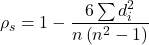
$\begin{align*} \rho_{s} = 1 - \frac{6 \sum d_{i}^2}{n \left (n^2 - 1 \right )} \end{align*}$

where d_i is the difference between the ranks of X₁ and X₂ for each experimental unit. This formula assumes that there are no tied ranks; if there are, use the equation for the product moment correlation instead (but on the ranks).

R commander has an option to calculate the Spearman rank correlation simply by selecting the check box in the correlation sub menu. However, if the data set is small, it may be easier to just run the correlation in the script window.

Our example for the product moment correlation was between Drosophila fly wing length and wing area (Table 1).

Table 1. Fly wing lengths and area, units mm and mm², respectively (Dohm pers obs.)

Obs	Student	Length	Area
1	S01	1.524	0.446
2	S01	2.202	0.876
3	S01	1.52	0.39
4	S01	1.62	0.51
5	S01	1.71	0.736
6	S03	1.551	0.453
7	S03	2.228	0.882
8	S03	1.46	0.394
9	S03	1.659	0.503
10	S03	1.719	0.535
11	S05	1.534	0.441
12	S05	2.223	0.889
13	S05	1.49	0.391
14	S05	1.633	0.514
15	S05	1.704	0.546
16	S08	1.551	0.453
17	S08	2.228	0.882
18	S08	1.468	0.394
19	S08	1.659	0.503
20	S08	1.719	0.535

Repeated observations by image analysis (ImageJ) were collected by four students (S01, S03, So5, S08) from fixed wings to glass slides.

Here’s the scatterplot of the ranks of fly wing length and fly wing area (Fig 1).

fly wings, area by length
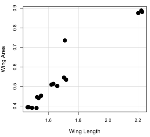
Figure 1. Drosophila wing area (mm²) by wing length (mm).

A nonparametric alternative to the product moment correlation, the Spearman Rank correlation can be obtained directly. The Spearman correlation involves ranking the data, ie, converting data types, from ratio scale data to ordinal scale, then applying the same formula used for the Product moment correlation to the ranked data. The Spearman correlation would be the choice for testing linear association between two ordinal type variables. It is also appropriate in lieu of the parametric product moment correlation when the statistical assumptions are not met, eg, normality assumption.

R code

For the Spearman rank correlation, at the R prompt type

cor.test(Area, Length, alternative="two.sided", method="spearman")

R returns with
    Spearman's rank correlation rho

data:  Area and Length
S = 58.699, p-value = 5.139e-11
alternative hypothesis: true rho is not equal to 0
sample estimates:
      rho 
0.9558658

Alternatively, to calculate either correlation, use R Commander.

Rcmdr: Statistics → Summaries→ Correlation test

Example

BM=c(29,29,29,32,32,35,36,38,38,38,40)
Matings=c(0,2,4,4,2,6,3,3,5,8,6)

cor.test(BM,Matings, method="spearman")
Warning in cor.test.default(BM, Matings, method = "spearman") :
  Cannot compute exact p-value with ties

        Spearman's rank correlation rho

data:  BM and Matings
S = 77.7888, p-value = 0.03163
alternative hypothesis: true rho is not equal to 0
sample estimates:
      rho 
0.6464143

cor.test(BM,Matings, method="pearson")

        Pearson's product-moment correlation

data:  BM and Matings
t = 2.6728, df = 9, p-value = 0.02551
alternative hypothesis: true correlation is not equal to 0
95 percent confidence interval:
 0.1087245 0.9042515
sample estimates:
      cor 
0.6652136

Other correlations

Kendall’s tau

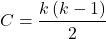
Another nonparametric correlation is Kendall’s tau (τ). Rank the X₁ values, then rank the X₂ values. Count the number of X₁, X₂ pairs that have the same rank (concordant pairs) and the number of X₁, X₂ pairs that do not have the same rank (discordant pairs), Kendall’s tau is then

$\begin{align*} \tau = \frac{\left ( no. \ of \ concordant \ pairs \right ) - \left ( no. \ of \ discordant \ pairs \right ) }{\frac{1}{2} \left ( n - 1 \right )} \end{align*}$

where n is the number of pairs.

Note 1: The denominator is our familiar number of pairwise comparisons if we take k = n

$\begin{align*} C = \frac{k \left ( k - 1 \right )}{2} \end{align*}$

We introduced concordant and discordant pairs when we presented McNemar’s test and cross-classified experimental design in Chapter 9.6.

Example: Judging of Science Fair posters

What is the agreement between two judges, A and B, who evaluated the same science fair posters? Posters were evaluated on if the student’s project was hypothesis-based and judges used a Likert-like scale Strongly disagree (1), Somewhat disagree (2), Neutral (3), Somewhat agree (4), Strongly agree (5).

Table 2. Two judges evaluated six posters for evidence of hypothesis-based project

Poster	Judge.A	Judge.B
1	5	4
2	2	3
3	4	2
4	3	1
5	2	1
6	4	3

A concordant pair represents a poster ranked higher by both judges, while a discordant pair is a poster ranked high by one judge but low by another judge. Poster 1 and poster 5 were concordant pairs,

In R, it is simple to get this correlation directly by invoking the cor.test function and specifying the method equal to kendall. The cor.test assumes that the data are in a matrix, so use the cbind function to bind two vectors together – note the vectors need to have the same number of observations. If the data set is small, it is easier to just enter the data directly in the script window of R commander.

A = c(2,2,3,4,4,5)
B = c(1,3,1,2,3,4)
m = cbind(A,B)
cor.test(A,B, method="kendall")

  Cannot compute exact p-value with ties

        Kendall's rank correlation tau

data:  A and B
z = 1.4113, p-value = 0.1581
alternative hypothesis: true tau is not equal to 0
sample estimates:
      tau 
0.5384615

End of R output

There were no ties in this data set, but we can run the product moment correlation just for comparison

cor.test(A,B, method="pearson")

        Pearson's product-moment correlation

data:  A and B
t = 1.4649, df = 4, p-value = 0.2168
alternative hypothesis: true correlation is not equal to 0
95 percent confidence interval:
 -0.4239715  0.9478976
sample estimates:
      cor 
0.5909091

End R output

Tetrachoric and Polychoric correlation

Tetrachoric correlations used for binomial outcomes (yes, no), polychoric correlation used for ordinal categorical data like the Likert scale. Introduced by Karl Pearson, commonly applied correlation estimate for Item Analysis in psychometric research. Pyschometrics, a sub-discipline within psychology and now a significant part of education research, is about evaluating assessment tools.

R package psych.

R code: Tetrachoric correlation

tetrachoric(x,y=NULL,correct=.5,smooth=TRUE,global=TRUE,weight=NULL,na.rm=TRUE,
     delete=TRUE)

R code: Polychoric correlation

polychoric(x,smooth=TRUE,global=TRUE,polycor=FALSE,ML=FALSE, std.err=FALSE, 
     weight=NULL,correct=.5,progress=TRUE,na.rm=TRUE,  delete=TRUE)

Polyserial correlation

R package polychor. Used to estimate linear association between a ratio scale variable and an ordinal variable.

R code: Polyserial correlation

polyserial(x,y)

Biserial correlation would be a special case of the polyserial correlation, where ordinal variable is replaced by a dichotomous (binomial) variable.

R code: Polyserial correlation

biserial(x,y)

Intra-class correlation coefficient

Both the ICC and the product moment correlation, r, which we introduced in Chapter 16.1, are measures of strength of linear association between two ratio scale variables (Jinyuan et al 2016). But ICC is more appropriate for association between repeat measures of the same thing, eg, repeat measures of running speed. In contrast, the product moment correlation can be used to describe association between any two variables, eg, between repeat measures of running speed, but also between say running speed and maximum jumping height. ICC is used when quantitative measures are organized into paired groups, eg, before and after on same subjects, or cross-classified designs. ICC was introduced in Chapter 12.3 as part of discussion of repeated measures and random effects. ICC is used extensively to assess reliability of a measurement instrument (Shrout and Fleiss 1979; McGraw and Wong 1996).

Example. Data from Table 2

library(psych)
ICC(myJudge, lmer=FALSE)

R output follows

Intraclass correlation coefficients 
                         type  ICC   F df1 df2      p lower bound upper bound
Single_raters_absolute   ICC1 0.40 2.3   5   6  0.166      -0.306        0.84
Single_random_raters     ICC2 0.46 3.9   5   5  0.081      -0.093        0.85
Single_fixed_raters      ICC3 0.59 3.9   5   5  0.081      -0.130        0.90
Average_raters_absolute ICC1k 0.57 2.3   5   6  0.166      -0.880        0.91
Average_random_raters   ICC2k 0.63 3.9   5   5  0.081      -0.205        0.92
Average_fixed_raters    ICC3k 0.74 3.9   5   5  0.081      -0.299        0.95

Number of subjects = 6 Number of Judges = 2
See the help file for a discussion of the other 4 McGraw and Wong estimates

Lots of output, lots of “ICC”. However, rather than explaining each entry, reflect on the type and review the data. Were the posters evaluated repeatedly? Posters were evaluated twice, but only once per judge, so there is a repeated design with respect to the posters. Had the judges been randomly selected from a population of all possible judges? No evidence was provided to suggest this, so judges were a fixed factor (see Chapter 12.3 and Chapter 14.3).

The six ICC estimates reported by R follow discussion in Shrout and Fliess (1979), and our description fits their Case 3: “Each target is rated by each of the same k judges, who are the only judges of interest (p. 421)” Thus, we find ICC for single fixed rater, ICC = 0.59. Note that we would fail to reject the hypothesis that the judges evaluations were associated.

Questions

1. Write up three learning outcomes for this page. Hint: Point your favorite generative AI to this page and ask for help.

2. See Homework 10, Mike’s Workbook for biostatistics

Quiz Chapter 16.4

Spearman and other correlations

Chapter 16 contents

16.1 – Product moment correlation

Introduction
The correlation coefficient
Effect size
Standard error of the correlation
Confidence interval
Significance testing
R code
Assumptions of the product-moment correlation
Testing two independent correlations
Questions
Quiz
Chapter 16 contents

Introduction.

A correlation is used to describe the direction $\pm$ magnitude of linear association and the between two variables. There are many types of correlations, some are based on ranks, but the one most commonly used is the product-moment correlation (r). The Pearson product-moment correlation is used to describe association between continuous, ratio-scale data, where “Pearson” is in honor of Karl Pearson (b 1857 – d. 1936).

There are many other correlations, including Spearman’s and Kendall’s tau (τ) (Chapter 16.4) and ICC, the intraclass correlation (Chapter 12.3 and Chapter 16.4).

The product moment correlation is appropriate for variables of the same kind — for example, two measures of size, like the correlation between body weight and brain weight.

Spearman’s and Kendall’s tau correlation are nonparametric and would be alternatives to the product moment correlation. The intraclass correlation, or ICC, is a parametric estimate suitable for repeat measures of the same variable.

The correlation coefficient.

$\begin{align*} r_{XY}=\frac{\sum_{i=1}^{n}\left (X_{i}-\bar{X} \right )\left (Y_{i}-\bar{Y} \right )}{\left (n-1 \right )s_{X} s_{Y}} \end{align*}$

The numerator is the sum of products and it quantifies how the deviates from X and Y means covary together, or change together. The numerator is known as a “covariance.”

$\begin{align*} COV_{XY}=\sum_{i=1}^{n}\left (X_{i}-\bar{X} \right )\left (Y_{i}-\bar{Y} \right ) \end{align*}$

The denominator includes the standard deviations of X and Y; thus, the correlation coefficient is the standardized covariance.

The product moment correlation, r, is an estimate of the population correlation, ρ (pronounced rho), the true relationship between the two variables.

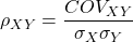
$\begin{align*} \rho_{XY}=\frac{COV_{XY}}{\sigma_{X} \sigma_{Y}} \end{align*}$

where COV(X,Y) refers to the covariance between X and Y.

Effect size.

Estimates for r range from -1 to +1; the correlation coefficient has no units. A value of 0 describes the case of no statistical correlation, ie, no linear association between the two variables. Usually, this is taken as the null hypothesis for correlation — “No correlation between two variables,” with the alternative hypothesis (2-tailed) — “There is a correlation between two variables.”

Like mean difference effect size, we can report the strength of correlation between two variables. Consider the magnitude and not the direction $\pm$ . Like Cohen’s effect size:

Absolute value	Magnitude of association
0.10	small, weak
0.30	moderate
> 0.50	strong, large

Note that one should not interpret a “strong, large” correlation as evidence that the association is necessarily real. See Ch16.c for more on spurious correlations.

Standard error of the correlation.

An approximate standard error for r can be obtained using this simple formula

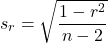
$\begin{align*} s_{r}=\sqrt{\frac{1-r^2}{n-2}} \end{align*}$

This standard error can be used for significance testing with the t-test. See below.

Confidence interval.

Like all situations in which an estimate is made, you should report the confidence interval for r. The standard error approximation is appropriate when the hull hypothesis is $r = 0$ , because the joint distribution is approximately normal. However, as the estimate approaches the limits of the closed interval $(-1,1)$ , the distribution becomes increasingly skewed.

The approximate confidence interval for the correlation is based on Fisher’s z-transformation. We use this transformation to stabilize the variance over the range of possible values of the correlation and, therefore, better meet the assumptions of parametric tests based on the normal distribution.

The transform is given by the equation

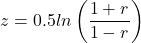
$\begin{align*} z= 0.5 ln\left ( \frac{1+r}{1-r} \right ) \end{align*}$

where ln is the natural logarithm. In the R language we get the natural log by log(x), where x is a variable we wish to transform.

Equivalently, z can be rewritten as

$\begin{align*} z= arctanh\left (r \right ) \end{align*}$

the inverse hyperbolic tangent function. In R language this function is called by atanh(r) at the R prompt.

The standard error for z is about

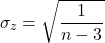
$\begin{align*} \sigma_{z} =\sqrt{\frac{1}{n-3}} \end{align*}$

We take z to be the estimate of the population zeta, ζ. We take the sampling distribution of z to be approximately normal and thus we may then use the normal table to generate the 95% confidence interval for zeta.

$\begin{align*} z-1.96\sigm_{z}\ < \ \zeta \ < \ z+1.96\sigm_{z} \end{align*}$

Why 1.96? We want 95% confidence interval, so that at Type I α = 0.05, we want the two tails of the Normal distribution (see Appendix 20.1), or + 0.025. Thus +0.025 is +1.96 and -1.96 corresponds to 0.025 (α = 0.05/2 tails = 0.025).

Significance testing.

Significance testing of correlations is straightforward, with the noted caveat about the need to transform in cases where the estimate is close to $\pm1$ . For the typical test of null hypothesis, the correlation, r, is equal to 0, the t distribution can be used (ie, it’s a t-test).

$\begin{align*} t=\frac{r-0}{s_{r}} \end{align*}$

which has degrees of freedom, DF = n – 2.

Use the t-table critical values to test the null hypothesis involving product moment correlation (eg, Appendix 20.3; for Spearman rank correlation $r_{s}$ , see Table G, p. 686 in Whitlock & Schluter).

Alternatively (and preferred), we’ll just use R and Rcmdr’s facilities without explanation; the t distribution works OK as long as the correlations are not close to $\pm1$ , in which case other things need to be done — and this is also true if you want to calculate a confidence interval for the correlation.

You are sufficiently skilled at this point to evaluate whether a correlation is statistically significantly different from zero — just check out whether the associated P-value is less than or greater than alpha (usually set at 5%). A test of whether or not the correlation, r₁, is equal to some value, r₂, other than zero is also possible. For an approximate test, replace zero in the above test statistic calculation with the value for r₂, and calculate the standard error of the difference. Note that use of the t-test for significance testing of the correlation is an approximate test — if the correlations are small in magnitude using the Fisher’s Z transformation approach will be less biased, where the test statistic z now is

$\begin{align*} \z =\frac{z_{r1} - z_{r2}}{\sigma_{z1-z2}} \end{align*}$

and standard error of the difference is

$\begin{align*} \sigma_{z1-z2} =\sqrt{\frac{1}{n1-3}+\frac{1}{n2-3}} \end{align*}$

and look up the critical value of z from the normal table.

R code.

To calculate correlations in R and Rcmdr, have ratio-scale data ready in the columns of a R and Rcmdr data frame. We’ll introduce the commands with an example data set from my genetics laboratory course.

Question. What is the estimate of the product moment correlation between Drosophila fly wing length and area?

Data (thanks to some of my genetics students!)

Area <- c(0.446, 0.876, 0.390, 0.510, 0.736, 0.453, 0.882, 0.394, 0.503, 0.535, 0.441, 0.889, 0.391, 0.514, 0.546, 0.453, 0.882, 0.394, 0.503, 0.535)
Length <- c(1.524, 2.202, 1.520, 1.620, 1.710, 1.551, 2.228, 1.460, 1.659, 1.719, 1.534, 2.223, 1.490, 1.633, 1.704, 1.551, 2.228, 1.468, 1.659, 1.719)

Create your data frame, eg,

FlyWings <- data.frame(Area, Length)

And here’s the scatterplot (Fig 1). We can clearly see that Wing Length and Wing Area are positively correlated, with one outlier (Fig 1).

fly wings, area by length

Figure 1. Scatterplot of Drosophila wing area by wing length.

The R command for correlation is simply cor(x,y). This gives the “pearson” product moment correlation, the default. To specify other correlations, use method = "kendall", or method = "spearman" (See Chapter 16.4).

Question. What are the Pearson, Spearman, and Kendall’s tau estimates for the correlation between fly Wing Length and Wing Area?

At the R prompt, type

cor(Length,Area) 
[1] 0.9693334 
cor(Length,Area, method="kendall") 
[1] 0.8248008 
cor(Length,Area, method="spearman") 
[1] 0.9558658

Note that we entered Length first. On your own, confirm that the order of entry does not change the correlation estimate. To both estimate test the significance of the correlation between Wing Area and Wing Length, at the R prompt type

cor.test(Area, Length, alternative="two.sided", method="pearson")

R returns with

Pearson's product-moment correlation 

data: Area and Length 

t = 16.735, df = 18, p-value = 2.038e-12>
alternative hypothesis: true correlation is not equal to 0
95 percent confidence interval:
0.9225336 0.9880360
sample estimates:
   cor
0.9693334

Alternatively, to calculate and test the correlation, use R Commander, Rcmdr: Statistics → Summaries→ Correlation test

Note 1. R’s cor.test uses Fisher’s z transformation; note if we instead use the approximate calculation instead how poor the approximation works in this example. The estimated correlation was 0.97, thus the approximate standard error was 0.058. The confidence interval (t-distribution, alpha=0.05/2 and 18 degrees of freedom) was between 0.848 and 1.091, which is greater than the z transform result and returns an out-of-bounds upper limit.

Alternative packages to base R provide more flexibility and access to additional approaches to significance testing of correlations (Goertzen and Cribbie 2010). For example, z_cor_test() from the TOSTER package.

z_cor_test(Area, Length)

Pearson's product-moment correlation
data:  Area and Length
z = 8.5808, N = 20, p-value < 2.2e-16
alternative hypothesis: true correlation is not equal to 0
95 percent confidence interval:
0.9225336 0.9880360
sample estimates:
      cor
0.9693334

To confirm, check the critical value for z = 8.5808, two-tailed, with

> 2*pnorm(c(8.5808), mean=0, sd=1, lower.tail=FALSE)
[1] 9.421557e-18

Note the difference is that Fisher’s z is used for hypothesis testing; cor.test and z_cor_test return same confidence intervals.

and by bootstrap resampling (see Chapter 19.2),

boot_cor_test(Area, Length)

Bootstrapped Pearson's product-moment correlation

data: Area and Length
N = 20, p-value < 2.2e-16
alternative hypothesis: true correlation is not equal to 0
95 percent confidence interval:
0.8854133 0.9984744
sample estimates:
cor
0.9693334

The z-transform confidence interval would be preferred over the bootstrap confidence interval because it is narrower.

Assumptions of the product-moment correlation.

Interestingly enough, there are no assumptions for estimating a statistic. You can always calculate an estimate, although of course, this does not mean that you have selected the best calculation to describe the phenomenon in question, it just means that assumptions are not applicable for estimation. Whether it is the sample mean or the correlation, it is important to appreciate that, look, you can always calculate it, even if it is not appropriate!

Statistical assumptions and those technical hypotheses we evaluate apply to statistical inference — being able to correctly interpret a test of statistical significance for a correlation estimate depends on how well assumptions are met. The most important assumption for a null hypothesis test of correlation is that samples were obtained from a “bivariate normal distribution.” It is generally sufficient to just test normality of the variables one at a time (univariate normality), but the student should be aware that testing the bivariate normality assumption can be done directly (eg, Doornick and Hansen 2008).

Testing two independent correlations

Extending from a null hypothesis of the correlation is equal to zero to the correlation equals a particular value should not be a stretch for you. For example, since we use the t-test to evaluate the null hypothesis that the correlation is equal to zero, you should be able to make the connection that, like the two sample t-test, we can extend the test of correlation to any value. However, using the t-test without considering the need to stabilize the variance.

When two correlations come from independent samples, we can test whether or not the two correlations are equal. Rather than use the t-test, however, we use a modification of Fisher’s Z transformation. Calculate z for each correlation separately, then use the following equation to obtain Z. We then look up Z from our table of standard normal distribution (Appendix 20.1, or better — use the normal distribution functions in Rcmdr) and we can obtain the p-value of the test of the hypothesis that the two correlations are equal.

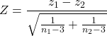
$\begin{align*} Z= \frac{z_{1}-z_{2}}{\sqrt{\frac{1}{n_{1}-3}+\frac{1}{n_{2}-3}}} \end{align*}$

Example. Two independent correlations are r1 = 0.2 and r2 = 0.34. Sample sizes for group 1 was 14 and for group 2 was 21. Test the hypothesis that the two correlations are equal. Using R as a calculator, here’s what we might write in the R script window and the resulting output. It doesn’t matter which correlation we set as r1 or r2, so I prefer to calculate the absolute value of Z and then get the probability from the normal table for values greater or equal to |Z| (ie, the upper tail).

z1 = atanh(0.2)
z2 = atanh(0.34)
n1 = 14
n2 = 21
Z = abs((z1-z2)/sqrt((1/(n1-3))+(1/(n2-3))))
Z = 0.3954983

From the normal distribution table we get a p-value of 0.3462 for the upper tail. Because this p-value is not less than our typical Type I error rate of 0.05, we conclude that the two correlations are not in fact significantly different.

Rcmdr: Distributions → Continuous distributions → Normal distribution → Normal probabilities…

pnorm(c(0.3954983), mean=0, sd=1, lower.tail=FALSE)

R returns

[1] 0.3462376

To make this two-tailed, of course all we have to do is multiple the one-tailed p-value by two, in this case two-tailed p-value = 0.69247.

Write a function in R

There’s nothing wrong with running the calculations as written. But R allows users to write their own functions. Here’s one possible function we could write to test two independent correlations. Write the R function in the script window.

test2Corr = function(r1,r2,n1,n2) {
z1=atanh(r1); z2=atanh(r2)
Z = abs((z1-z2)/sqrt((1/(n1-3))+(1/(n2-3))))
pnorm(c(Z), mean=0, sd=1, lower.tail=FALSE)
}

After submitting the function, we then invoke the function by typing at the R prompt

p = test2Corr(0.2,0.34,14,21); p

Again, R returns the one-tailed p-value

[1] 0.3462376

Unsurprisingly, these simple functions are often available in an R package. In this case, the psych package provides a function called r.test() which will accommodate the test of the equality hypothesis of two independent correlations. Assuming that the psych package has been installed, at the R prompt we type

require(psych)
r.test(14,.2,.34,n2=21,twotailed=TRUE)

And R returns

Correlation tests
Call:r.test(n = 14, r12 = 0.20, r34 = 0.34, n2 = 21, twotailed = TRUE)
Test of difference between two independent correlations
z value 0.4 with probability 0.69

More on testing correlations

The discussion above, as stated, assumes the two correlations are independent of each other. In ecological studies, for example, it is not uncommon to have estimates for correlations among multiple pairs of traits. Thus, our approach would not be appropriate for testing whether the difference in correlations between body mass/ornament size and body mass/swimming performance of male killifish because both correlations include the same variable (body mass). A better solution would be to use William’s t-test (Williams 1959, Diedenhofen and Musch 2015).

Note 2: This example was selected from Sowersby et al 2022 — I’m not implying here that the authors analyzed their results incorrectly, I just like the example of traits to illustrate the point!

The null hypothesis was evaluated using Williams’ (1959) $t$ -test for overlapping dependent correlations with $df = n - 3$ degrees of freedom, calculated as:

(1) $\begin{equation*} t = (r_{12} - r_{13}) \sqrt{\frac{(n - 1)(1 + r_{23})}{2 \cdot \left(\frac{n - 1}{n - 3}\right) |R| + \frac{(r_{12} + r_{13})^2}{4} (1 - r_{23})^3}} \end{equation*}$

Where $|R|$ represents the determinant of the $3 \times 3$ correlation matrix, defined as:

(2) $\begin{equation*} |R| = 1 - r_{12}^2 - r_{13}^2 - r_{23}^2 + 2r_{12}r_{13}r_{23} \end{equation*}$

The r.test() in psyche package can be modified to handle this. R code for a made up example:

# 1. Define your sample size (N)
sample_size <- 65 # Example: 65 male killifish

# 2. Define the three correlation coefficients (r)
# r12 = correlation between body mass and ornament size
# r13 = correlation between body mass and swimming performance
# r23 = correlation between ornament size and swimming performance
r_mass_ornament <- 0.55
r_mass_swim <- 0.30
r_ornament_swim <- 0.40

# 3. Run Williams' t-test using r.test()
result <- psych::r.test(
   n = sample_size,
   r12 = r_mass_ornament,
   r13 = r_mass_swim,
  r23 = r_ornament_swim
)

# 4. View the results
print(result)

R output

Correlation tests 
Call:[1] "r.test(n = 65 , r12 = 0.55 , r23 = 0.4 , r13 = 0.3 )"
Test of difference between two correlated correlations 
t value 2.13 with probability < 0.037NULL

And we would conclude that the two correlations are indeed statistically different from each other.

Alternatively, use the cocor.dep.groups.overlap() from the cocor package. This generates all of the proposed tests of such correlations.

For our example then,

library(cocor)

# 1. Define sample size (N)
sample_size <- 65
# 2. Define individual correlations (r)
# r.jk = correlation between body mass (j) and ornament size (k)
# r.jh = correlation between body mass (j) and swimming performance (h)
# r.kh = correlation between ornament size (k) and swimming performance (h)
r_mass_ornament <- 0.55
r_mass_swim <- 0.30
r_ornament_swim <- 0.40
#3. Note: j is the overlapping/shared variable (body mass)
my_result <- cocor.dep.groups.overlap(
    r.jk = r_mass_ornament,
    r.jh = r_mass_swim,
   r.kh = r_ornament_swim,
   n = sample_size,
   alternative = "two.sided",
   alpha = 0.05
)

# 4. View the full comparison report
show(my_result)

Note 3: To extract and print ONLY Williams’ t-test results use my_results@williams1959.

R output (rearranged, brought William’s t-test up to the top for comparisons).

Results of a comparison of two overlapping correlations based on dependent groups

Comparison between r.jk = 0.55 and r.jh = 0.3
Difference: r.jk - r.jh = 0.25
Related correlation: r.kh = 0.4
Group size: n = 65
Null hypothesis: r.jk is equal to r.jh
Alternative hypothesis: r.jk is not equal to r.jh (two-sided)
Alpha: 0.05

williams1959: Williams' t (1959)
t = 2.1291, df = 62, p-value = 0.0372
Null hypothesis rejected

pearson1898: Pearson and Filon's z (1898)
z = 2.1217, p-value = 0.0339
Null hypothesis rejected

hotelling1940: Hotelling's t (1940)
t = 2.1635, df = 62, p-value = 0.0344
Null hypothesis rejected

olkin1967: Olkin's z (1967)
z = 2.1217, p-value = 0.0339
Null hypothesis rejected

dunn1969: Dunn and Clark's z (1969)
z = 2.0926, p-value = 0.0364
Null hypothesis rejected

hendrickson1970: Hendrickson, Stanley, and Hills' (1970) modification of Williams' t (1959)
t = 2.1635, df = 62, p-value = 0.0344
Null hypothesis rejected

steiger1980: Steiger's (1980) modification of Dunn and Clark's z (1969) using average correlations
z = 2.0795, p-value = 0.0376
Null hypothesis rejected

meng1992: Meng, Rosenthal, and Rubin's z (1992)
z = 2.0675, p-value = 0.0387
Null hypothesis rejected
95% confidence interval for r.jk - r.jh: 0.0161 0.6017
Null hypothesis rejected (Interval does not include 0)

hittner2003: Hittner, May, and Silver's (2003) modification of Dunn and Clark's z (1969) using a backtransformed average Fisher's (1921) Z procedure
z = 2.0741, p-value = 0.0381
Null hypothesis rejected

zou2007: Zou's (2007) confidence interval
95% confidence interval for r.jk - r.jh: 0.0155 0.4877
Null hypothesis rejected (Interval does not include 0)

Note 4: show() not summary() because cocor.dep.groups.overlap() returns an S4 object.

Questions

Write up three learning outcomes for this page. Hint: Point your favorite generative AI to this page and ask for help.
True or False. Generally, the null hypothesis of a test of a correlation is Ho: r = 0, although in practice, one could test a null of r = any value.
Return to the fly wing example. What was the estimate of the value of the product moment correlation? The Spearman Rank correlation? The Kendall’s tau?
OK, you have three correlation estimates for test of the same null hypothesis, ie, correlation between Length and Area is zero. Which estimate is the best estimate?
Apply the Fisher z transformation to the estimated correlation, what did you get?
For the fly wing example, what were the degrees of freedom?
For the fly wing example, calculate the approximate standard error of the product moment correlation.
Return one last time to the fly wing example. What was the value of the lower limit of the 95% confidence interval for the estimate of the product moment correlation? And the value of the upper limit?
Assume that another group of students (n = 15) made measurements on fly wings and the correlation was 0.86. Is the difference between the two correlations for the two groups of students equal? Obtain the probability using the Z calculation and R (Chapter 6.7) or the normal table.

Quiz Chapter 16.1

Product moment correlation