5.6 – Sampling from Populations
Introduction
Researchers generally can’t study an entire population. More generally, striving to study each member of a population is not necessary to arrive at answers about the population. For example, consider the question, does taking a multivitamin daily improve health? What are our options? Do we really need to follow every single individual in the United States of America, monitoring their health and noting whether or not the person takes vitamins daily in order to test (inference) this hypothesis? Or, can we get at the same answer by careful experimental design (see Schatzkin et al 2002; Dawsey et al 2014)? Supplement use is wide-spread in the United States, but both health and vitamin use differ by demographics. Young people tend to be healthier than older people and older people tend to take supplements more than younger people.
A subset of the population is measured for some trait or characteristic. From the sample, we hope to refer back to the population. We want to move from anecdote (case histories) to possible generalizations of use to the reference population (all patients with these symptoms). How we sample from the reference population limits our ability to generalize. We need a representative sample: simple to define, hard to achieve.
Statistics becomes necessary if we want to infer something about the entire populations. (Which is usually the point of doing a study!!) Typically tens to thousands of individuals are measured. But in addition, HOW we obtain the sample of individuals from the reference population is CRITICAL.
Kinds of sampling include (adapted from Box 1, Tyrer and Heyman 2016; see also McGarvey et al 2016)
Probability sampling
- random
- stratified
- blocking
- clustered
- systematic
Nonprobability sampling
- convenience, haphazard
- judgement
- quota
- snowball
For an exhaustive, authoritative look at sampling, see Thompson (2012).
How can samples be obtained?
Sampling from a population may be convenient. For one famous example, consider the Bumpus data set. (We introduced this data set in Question 5, Chapter 5.) So the legend goes, Professor Bumpus was walking across the campus of Brown University, the day after a severe winter storm, and came across a number of motionless house sparrows on the ground. Bumpus collected the birds and brought them to his lab. Seventy-two birds recovered; 64 did not (Table1).
Table 1. A subset of Bumpus data set, summarized by sex of birds.
| House sparrows | Lived | Died |
|---|---|---|
| Female | 21 | 28 |
| Male | 51 | 36 |
Bumpus reported differences in body size that correlated with survival (Bumpus 1899), and this report is often taken as an example of Natural Selection (cf. Johnston et al 1972). The Bumpus dataset is clearly convenience sampling. It’s also a case study: a report of a single incident. But given that is is a large sample (n = 136), it is tempting to use the data to inform about about possible characteristics of the birds that survived compared with those that perished.
Another way we collect samples from populations is best termed haphazard. In graduate school I got the opportunity to study locomotor performance of whiptail lizards (Aspidoscelis tigris, A. marmoratus, genus formerly Cnemidophorus**) across a hybrid zone in the Southwest United States (Dohm et al. 1998). During the day we would walk in areas where the lizards were known to occur and capture any individual we saw by hand. (This would sometimes mean sticking our hands down into burrows, which was always exciting — you never really knew if you were going to find your lizard or if you were going to find a scorpion, venomous spider, or …) Lizards collected were returned to the lab for subsequent measures. Clearly, this was not convenience sampling; it involved a lot of work under the hot sun. But just as clearly, we could only catch what we could see and even the best of us would occasionally lose a lizard that had been spotted. Moreover, one suspects we missed many lizards that were present, but not in our view. Lizards that were underground at the time we visited a spot would not be seen nor captured by us; individual lizards that were especially wary of people (Bulova 1994) would also escape us. In other words, we caught the lizards that were catchable and can only assume (hope?) that they were representative of all of these lizards. Applying a grid or quadrant system to the area and then randomly visiting plots within the grid or quadrant might help, but still would not eliminate the potential for biased sampling we faced in this study.
Quota sampling implies selection of subjects by some specific criteria, weighted by the proportions represented in the population. It’s different from stratified sampling because there is no random selection scheme: subjects are selected based on matching some criteria, and collection for that group stops when the sample number matches the proportion in the population. Consider our vitamin supplement survey. If student population at Chaminade University was the reference population, and we have enough money to survey 100 students, then we would want a sample of 70 women students and 30 male students, representing the proportions of the student population.
Snowball sampling implies that you rely on word-of-mouth to complete sampling. After initial recruitment of subjects, sample size for the study increases because early participants refer others to the researchers. This can be a powerful tool for reaching underrepresented communities (eg, Valerio et al 2016).
Types of Probability sampling
Random sampling is an example of probability sampling. As we defined earlier, simple random sampling requires that you know how many subjects are in the population (N) and then each subject has an equal chance of being selected

Examples of nonprobability sampling include
- convenience sampling
- volunteer sampling
- judgement sampling
Convenience sampling (the first 20 people you meet at the library lanai); volunteer sampling (you stand in front of a room of strangers and ask for any ten people to come forward and take your survey — or more seriously, persons with a terminal disease calling a clinic reportedly known to cure the disease with a radical new, experimental treatment), and judgement sampling (to study tastes in fashion, you decide that only persons over six feet tall should be included because .…).
Random in statistics has a very important, strict meaning. As opposed to our day-to-day usage, random sampling from a population means that the probability that any one individual is chosen to be included in a sample is equal. Formally, this is called simple random sampling to distinguish it from more complex schemes. For a sampling procedure to be random requires a formal procedure for sampling a population with known size (N).
For example, at the end of the semester, I may select the order for student presentations at random. Thus, students in the classroom would be considered the population (groups of students are my sample unit, not individual students!). What is the probability that your group will be called first? Second? We need to know how many groups there are to conduct simple random sampling. Let’s take an extreme and say that all groups have a size of one; there are 26 students in this room, so

or

of being selected first.
Now to determine the probability of your group being selected second, we need to distinguish between two kinds of sampling:
- Sampling with replacement — after I select the first group, the first group is returned to the pool of groups that have not been selected. In other words, with replacement, your group could be selected first and selected second! The probability of being selected second then remains

.
- Sampling without replacement — after I select the first group, then I have

groups left to select the second group, so probability that your group will be second is

. The first group has already been selected and is not available.
Random sampling refers to how subjects are selected from the target, reference population. Random assignment, however, describes the process by which subjects are assigned to treatment groups of an experiment. Random sampling applies to the external validity of the experiment: to the extent that a truly random sample was drawn, then results may be generalized to the study population. Random assignment of subjects to treatment however makes the experiment internally valid: results from the experiment may be interpreted in terms of causality.
R code, sample without replacement
sample(26)
[1] 1 10 11 23 17 13 8 6 19 20 21 16 14 15 5 2 12 4 26 22 9 7 25 18 3 24
R code, sample with replacement
mySample <- sample(26, replace = TRUE); mySample
[1] 9 26 24 9 3 1 23 14 26 6 5 19 17 23 11 12 3 8 7 19 2 16 3 11 1 1
How many elements duplicated?
out <- duplicated(mySample); table(out)
out
FALSE TRUE
17 9
More on sampling in R discussed in Sampling with computers below.
Additional sampling schemes
Simple random sampling is not the only option, but in many cases it is the most desirable. Consider our multivitamin study again. Perhaps studying the entire USA population is a bit extreme. How about working from a list of AARP members, sending out questionnaires to millions of persons on this list, getting back about 20% of the questionnaires, sorting through the responses and identifying the respondent to diet categories and multivitamin use. The researchers had nearly 500,000 persons willing and able to participate in their prospective study (Schatzkin et al 2001; Dawsey et al 2014; Lim et al 2021). It’s an enormous study. But is this really much better than our described lizard experiment? Let’s count the ways: Not all older people are members of AARP (that 500,000? That’s less than 1% of the 50 and older persons in the USA); A large majority of AARP members did not return surveys; Some fraction of the returned surveys were not usable; How representative of diverse aged populations in the United States is AARP?
Simple random sampling may not be practical, particularly if sub-populations, or strata, are present and members of the different sub-populations are not available to the researcher in the same numbers. In ecology, habitat-use studies routinely need to account for the patchiness of the environment in space and time (Wiens 1976; Summerville and Crisp 2021). Thus, samples are drawn in such a way to represent the frequency within each sub-population.
For a simple example, researchers conducting a controlled breeding program of mice don’t use simple random sampling to choose pairs of mates; after all, random sampling without regard of sex of the mice would lead to some pairings of males only, or females only (Fig 1).
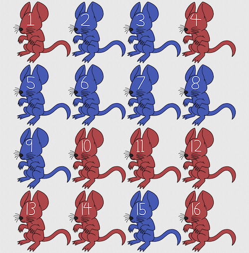
Figure 1. Sixteen mice, eight red and eight blue. Image © 2024 Mia D Graphics
R code
pairs <- c(rep("red", 8), rep("blue", 8))
replicate(2, sample(pairs, 8), simplify = FALSE)
[[1]]
[1] "blue" "blue" "blue" "red" "blue" "red" "blue" "red"

[[2]]
[1] "blue" "blue" "red" "red" "red" "red" "red" "blue"
Oops. If we interpret the output blue = male and red = female, then four out of the eight pairs were same sex pairings.
Thus, the breeding strategy is to random sample from female mice and from male mice and the stratification is sex of the mouse. Alternatively, breeders may select mice to form breeding pairs systematically: From a large colony with dozens of cages, the breeder may select one mouse from every third cage.
Stratified Random Sampling: Individuals in the population are classified into strata or sub-groups: age, economic class, ethnicity, gender, sex …, as many as needed. Then choose a simple random sample from each group, typically in proportion to the size of the sub-groups in the population. Combine those into the overall sample. For example, when I wanted a random sample of mice for my work, I called the supplier and requested that a total of 100 male and female mice be randomly selected from the five colonies they maintained. The reference population is the entire supply of mice at that company (at that time), but I wished to make sure that I got unrelated mice, so I needed to divide the population into groups (the five colonies) before my sample was constructed.
Note 1: The size of the population must be known in advance, just like in simplified random sampling. A more interesting example, the Social Security Administration conducts surveys of popular baby names by year. They post the top ten most popular names based on 1% or 5% (first strata), then by male/female (second strata).
For a simple example of the need for stratified sampling, consider our 16 blue and red mice again. If mice were randomly assigned to treatment group, then by chance unequal samples within strata may be assigned to a treatment group, potentially biasing our conclusions (Fig 2).
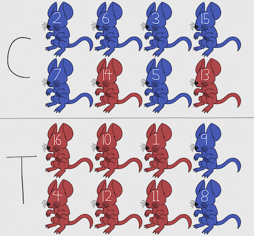
Figure 2. Sixteen mice, randomly assigned to treatment groups C and T; by chance, 75% blue in C and just 25% in T. If color was a confounding factor then our conclusions about the effectiveness of the treatment would be associated with color. Image © 2024 Mia D Graphics
Block sampling: superficially resembles stratified sampling, but refers to how experimental units are assigned to treatment groups. Blocks in experimental design refers to potentially confounding factors for which we wish to control, but are otherwise not interested in. For our example described in Figure 2, mouse color may not be of specific interest for our study and therefore would be considered a blocking effect.
Agricultural research provides a host of other blocking situations: plots distributed across an elevation or hydration gradient (Fig 3), soil types, and many others.

Figure 3. Agricultural fields in Central Poland. NASA https://visibleearth.nasa.gov/images/146593/agriculture-fields-in-central-poland/146595w
For a microbiology example, edge effects of heated culture plates. For a growth experiment it’s unlikely we are specifically interested in the plate layout on the growth characteristics of treated cells. However, it’s also unlikely we can assume placement has no influence on growth (eg, Mansoury et al 2021). A 96-well microplate has 60 inner wells and 36 edge wells (A1 – H1, A12-H12, plus 1st and 12th wells of columns B – H, for a total of 36 wells, Fig 4). Thus, analysis of growth effects should include a block effect for well position.
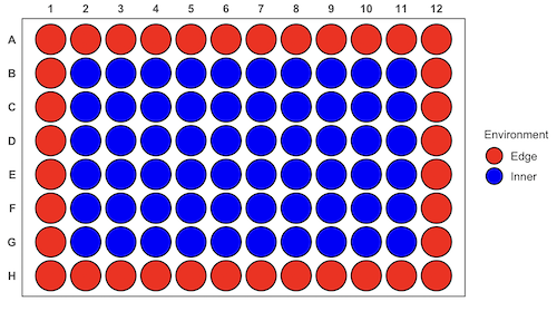
Figure 4. Format of 96-well plate. Red cells = “edge” wells; blue cells = “inner” wells. Plotted with ggplate package.
For long incubation periods it’s not unexpected that edge wells and inner wells may evaporate at different rates, potentially confounding interpretation of treatment effects if, by chance, treatment samples are more commonly assigned to edge wells. Block sampling implies subjects from treatment groups are randomly assigned to each block, in equal numbers if possible.
Cluster Sampling: In many situations, the population is far too large or too dispersed and scattered for a list of the entire population to be known. And, a random approach ignores that there is a natural grouping — people live next to each other, so there is going to be things in common. A multi-stage approach to sampling will be better than simply taking a random sample approach. Most surveys of opinion (when conducted reputably) use a multi-stage method. For example, if a senator wishes to poll his constituents about an issue, he may his pollster will randomly select a few of the counties from his state (first stage), then randomly select among towns or cities (second stage), to obtain a list of 1000 people to call. In some instances, they might use even more stages. At each stage, they might do a stratified random sample on sex, race, income level, or any other useful variable on which they could get information before sampling. If you are interested in this kind of work, for starters, see Couper and Miller (2009).
There are more types of sampling, and entire books written about the best way to conduct sampling. One important thing to keep in mind is that as long as the sample is large relative to the size of the population, each of the above methods generally will get the same answers (= the statistics generated from the samples will be representative of the population).
As long as some attempt is made to randomize, then you can say that the procedure is probability sampling. Nonprobability, or haphazard sampling, describes the other possibility, that is, each element is selected arbitrarily by a non-formal selecting of individual. … all the fish or birds that you catch may not be a random sample of those present in a population. For example,
- wild Pacific salmon do not feed on the surface, hatchery salmon feed on the surface. …
- all the individuals who respond to a survey.
- Phone surveys, web surveys, person on the street surveys… how random, how representative?
Sampling with computers
Now to determine the probability of your group being selected second, we need to distinguish between two kinds of sampling:
Sampling with replacement — after I select the first group, the first group is returned to the pool of groups that have not been selected. In other words, with replacement, your group could be selected first and selected second! The probability of being selected second then remains
Sampling without replacement — after I select the first group, then I have

groups left to select the second group, so probability that your group will be second is

. The first group has already been selected and is not available, and so on.
Sampling is usually easiest if a computer is used. Computers use algorithms to generate pseudo-random numbers. We call the resulting numbers pseudo-random to distinguish them from truly random physical processes (eg, radioactive decay). For more information about random numbers, please see random.org.
If all you wish to do is select a few observations or you need to use a random procedure to select subjects prior to observations, then these websites can provide a very quick, useful tool.
Sampling in Microsoft Excel or LibreOffice Calc
Microsoft’s Excel is pretty good at sampling, but requires knowledge of included functions. Here are the steps to generate random numbers and select with and without replacement in Excel. I’ll give you two cases.
1. For random numbers, enter the function =rand() in a cell, then drag the cell handle to fill in cells to N (in our case = 26, so A1 to A26). This function generates a random (more or less!) number between 0 and 1. We want digits between 1 and 26, not fractions between 0 and 1, so combine INT function with RAND function
=INT(27*RAND())
Note 2: To get between 1 and 9, multiply by 10 instead of 27; to get between 1 and 100, multiply by 101, etc.
In Excel to sample with replacement, simply pick the first two cells (the algorithm Excel used already has conducted sample with replacement. See next item for method to sample without replacement in Excel. You have to have installed the Data Analysis Tool Pak. Here’s instructions for Office 2010.
If you have a Mac and Office 2008, there is no Data Analysis Tool Pak, so to get this function in your Excel, install a third-party add-in program (eg, StatPlus, a free add-in, really nice, adds a lot of function to your Excel). If you have the 2011 version of Office for Mac, then the Data Analysis Tool Pak is included, but like your Windows counterparts, you have to install it (click here for instructions).
2. Let’s say that we have already given each group a number between 1 and 26 and we enter those numbers in sequence in column A.
To sample without replacement, select Tools → Data Analysis… (if this option is not available, you’ll have to add it — see Excel help for instructions, Fig 5).
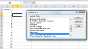
Figure 5. Screenshot of Sampling in Data Analysis menu, Microsoft Excel
Enter the cells with the numbers you wish to select from. In our example, column A has the numbers 1 through 26 representing each group in our class. I entered A:A as the Input Range.
Next, select “Random” and enter the number of samples. I want two.
Click OK and the output will be placed into cell B3 (my choice); I could have just as easily had Excel put the answer into a new worksheet.
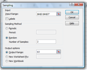
Figure 6. Screenshot of input required for Sampling in Data Analysis menu, Microsoft Excel
To sample with replacement from column A (with our 1 through 26), type in the formula B1
=INT(27*RAND())and the formula C1
=INDEX(A:A,RANK(B1,B:B))then drag the cell handles to fill in the columns (first column B, then column C).
That’ll do it for MS Excel or LibreOffice Calc.
Sampling with R (Rcmdr)
It’s much easier with much more control to get sampling in Rcmdr (R) than in Excel. Sampling in R is based on the function called sample() and sample.int(). I will present just the sample() command here.
sample(x, size, replace = FALSE, prob = NULL)Example
You want to sample ten integers between 1 and 10
sample(10)R output
sample(10)
[1]  5  1 10  8  7  3  4  9  2  6
You have a list of subjects, A1 through A10
subjects = c("A1","A2","A3","A4","A5","A6","A7","A8","A9","A10")
sample(subjects, 3, replace = FALSE, prob = NULL)
R output
sample(subjects, 3, replace = FALSE, prob = NULL)
[1] "A5" "A2" "A9"
Could use this to arrange random order for ten subjects
sample(subjects, 10, replace = FALSE, prob = NULL)
[1] "A9" "A3" "A8" "A2" "A1" "A4" "A10" "A7" "A5" "A6"
Try with replacement; To sample with replacement, type in TRUE after replace in the sample() function. The R output follows
sample(x, 10, replace = TRUE, prob = NULL)
[1]  5  5  3  5  3  7  3  5 10  6
R’s randomness is based on pseudonumbers and is, therefore, not truly random (actually, this is true of just about all computer-based algorithms unless they are based on some chaotic process). We can use this pseudo part to our advantage: if we want to reproduce our “random” process, we can seed the random number algorithm to a value (eg, 100), with the command in the Script Window
set.seed(100)For 10 random integers (eg, observations), type in the Script window
sample(10)R returns the following in the Output Window
sample(10)
[1] 4 5 7 3 10 9 2 1 6 8
Sampling was done without replacement. Here’s another selection round,
First without setting a seed value
sample(10)
[1] 10 4 7 3 8 1 2 9 6 5
Try again to see if get the same 10
sample(10)
[1]  1  4  8  2  9  6  5 10  3  7
Now to demonstrate how setting the seed allows you to draw repeated samples that are the same.
Note 3: If I need to precede the sample command with a set.seed() call, then sampling is repeatable.
set.seed(100)
sample(10)
[1] 4 3 5 1 9 6 10 2 8 7
and try again
set.seed(100)
sample(10)
[1] 4 3 5 1 9 6 10 2 8 7
Additional R packages that help with sampling schemes include: sampling() and spatialsample, which is part of the BiodiversityR package, which is available as a plugin for R Commander.
Quiz Chapter 5.6
Sampling from populations
Questions
- For our two descriptions of experiments in section 6.1 (the sample of patients; the sample of frogs), which sampling technique was used?
- What purpose is served by
set.seed()in a sampling trial? - Consider our question, Does taking a multivitamin daily improve health? Imagine you have a grant willing to support a long-term prospective study to follow up to one thousand people for ten years. List at least three concerns with proposed solutions about how sampling of subjects for the study.
- Imagine you wish to conduct a detailed survey to learn about student preferences. Your survey will include many questions, so you decide to ask just ten students. Student population is 70% female, 30% male.
- Assuming you select at random (simple random sampling), what is the chance that no male students will be included in your survey?
- You are able to increase the number of surveys to 20, 30, 40, or 50. What is the chance that no male students will be included in your survey for each of these increased sample numbers?
- What can you conclude about the effects of increasing survey sample size on representativeness of students for the survey?
- Discuss how you could apply a stratified sampling scheme to this survey and whether or not this approach improves representativeness.
- Why are random numbers generated by a computer called pseudo random numbers?
Chapter 5 contents
5 – Experimental design
Beyond numbers.
During this course, you will learn about statistics, yes, but my hope and goal for your experience in this class is much more than that: statistical reasoning. To have statistical reasoning skills, you need to be comfortable with the context of how data are acquired, ie, data acquisition. It’s not just about knowing how an instrument performs, eg, under or over the limits of quantification characteristics of the instrument lead to censored missing values, missing not at random (MNAR). In a broad stoke view, data are obtained from two kinds of studies: observational studies and experimental (manipulative) studies. what a correctly designed experiment can tell you about the world, and how a poorly designed experiment works against you. At the end of the semester, you should be familiar with the issues of Randomization, Control, Independence, and Replication.
The basics explained.
Experimental design is a discipline within statistics concerned with the analysis and design of experiments. Design is intended to help research create experiments such that cause and effect can be established from tests of the hypothesis. We introduced elements of experimental design in Chapter 2.4. I recommend a quick re-read: We talk about the different types of bias that can affect research. We also point out parts of the problem you’ll need to think about when planning a project, so you can avoid or reduce bias from the start.
Note 1: Just the highlights from Chapter 2.4: use randomization, blinding, and control measures in the study design. Different strategies may be needed depending on the type of bias.
Here, we expand our discussion of experimental design. We begin with review of definitions and an outline of an important concept in statistics. First, we need to be clear about why we measure or conduct experiments. We do so to collect data (datum is the singular) about a characteristic or trait from a population. Data are observations: they include observations and measurements from instruments. At their best, data are the “facts” of science.
Measurement, Observation, Variables, Values.
Measurement is how we as scientists acquire our data (Chapter 3.4). The process of measuring involves the assignment of numbers, codes, or labels to observations according to rules established prior to any data collection (Stevens 1946, Houle et al 2011). Observations refer to the units of measurement, whereas variables are the characteristics or traits that are measured. A value refers to the particular number, score, or label assigned to a particular sample for a variable. Variables are generic, the thing being measured, values are specific to the subject or sample being measured for the variable. Each discipline in biology has its own set of variables and samples may or may not have different values for each variable measured. Variables are summarized as a statistic (eg, the sample mean), which is a number taken to estimate a parameter, which pertains to the population. Variables and parameters in statistics were discussed in Chapter 3.4. Because numbers or scores or labels can be assigned according to different rules, this means that variables may be measured on different kinds of scales or data types. The different kinds of data types were presented in Chapter 3.1.
Missing values.
A missing value refers to lack of a value for an observation or variable (Chapter 3.5). Censored values, a type of missing value, include observations for which limited or partial information is available, eg, range, while a missing value lacks any information about the true value.
Missing values can affect analysis and many R algorithms are sensitive or may fail to run in the presence of missing values. Missing data may be of three kinds, and one of them, missing not at random (MNAR), can substantially influence the analysis. MNAR implies some observations are missing because of a systematic bias. Instrument limits of quantification are an example of systematic bias — for example, spectrophotometric absorbance readings of zero for a colorimetric assay (eg, Bradford protein assay) may not represent complete absence of the target, but rather, the lower detection limits of the instrument or the assay method (0.1 mg protein/mL in this case).
The other kinds of missing values are missing completely at random (MCAR) and missing at random (MAR). MCAR implies there is no association between any element of the experiment and the absence of a value. Analysis on MCAR data sets may support unbiased conclusions. MAR includes the random errors that occur during data acquisition: data may be lost because of operator error or power outage (shudder). Unlike MNAR, analysis of MAR, like MCAR data sets may still result in unbiased conclusions.
Note 2: The word “may” is doing some heavy lifting here; obviously, the size of the data set influences whether this claim holds.
One consequence of missing values — a decision how best to handle the lost information. The options are either pairwise deletion or listwise deletion. Listwise means the entire row, all variables, are lost for any record with one or more missing values. You recorded root length, stem length, numbers of secondary roots, time to germinate, but the SPAD meter failed and there is no chlorophyl reading for seedling #212? Sorry, the entire row is deleted. Optionally, the missing data is deleted pairwise — only chlorophyl reading for #212 is lost, all other variables remain.
Users of R will quickly learn some algorithms immediately fail to run if not instructed how to process missing values. In some cases, missing values can be replaced by imputed values.
Note 3: This being an introduction to applied biostatistics, we won’t dwell on the pros and cons of imputation. Instead, I point interested readers to two heavily cited articles: Schafer 1999; Schafer and Graham 2002.
Cause & Effect.
Observations or measurements gathered under controlled conditions (experiments) are essential if we are to answer questions about populations, to separate cause and effect, where one or more events is directly the result of another factor, as opposed to anecdote, a story about an event which, by itself, cannot be used to cause from association (eg, spurious correlations, see Ch 16.2). Recall that anecdotal evidence typically comes from personal experience, where observations may be obtained by non-systematic methods. Well designed experiments, in the classical sense, permit discrimination among competing hypotheses in large part because observations are collected according to strict rules. Well developed hypotheses tested by well-designed experiments permit ruling out alternative explanations (sensu Pratt [1964] strong inference). Observational studies, or epidemiology studies if we are talking about investigations of risk assessment, also may contribute to discussions of cause and effect (see history of smoking by Doll 1998).
Medicine is replete with stories about how a patient showed a particular set of symptoms, and how a physician applied a set of diagnostic protocols. An outcome was achieved, and the physician reports the outcome and circumstances related to the patient to her colleagues. This is an example of a case study, and the focus of investigation is the individual, the patient. The doctor’s report will sound like, “I tried the standard treatment given the diagnosis, and the patient’s symptoms diminished, but later returned. I tried a higher dose, but the patient’s symptoms persisted unabated.” No inferences are made to a wider set of individuals and the report is anecdotal. If observations are made on several patients, this may be a case series.
In ecology, a field biologist may notice a six-legged adult frog (Scott 1999, Alvarez et al 2021) — since frogs typically have four legs, the six-legged frog attracts the biologist’s eye and he jots down the circumstances in which the frog were found: relative humidity, air temperature, ground temperature, where the frogs was found (on lower leaf of a philodendron plant). A water source near where the frog was found is tested for pH with a meter the biologist carries, and a water sample is taken for later testing of herbicides. The frog is collected so that it can be checked for skin parasites. Upon further inspection, the frog did indeed have parasites known to cause deformities in other frog species. However, note that this example too, is a case study. Although the biologist makes additional observations, any conclusions about why the frog has six legs is anecdotal.
From these case studies, no conclusions can be drawn. We cannot say why the patient failed to respond to treatment, nor can we say why the frog has six legs. Why? Because these are singular events, and a variety of explanations can be given as to their causes — importantly, no controls are available, so there’s no way to distinguish among possibilities.
From such anecdotes, however, experiments can be designed. The physician may decide to recruit additional patients with the diagnosed illness and apply the standard treatment to see if her anecdote is a single, unique event, or more indicative of a problem with the treatment. The biologist may collect other frogs from the area near where he found the six-legged frog and check to see if they, too, have the parasites. If additional patients fail to respond to the treatment, then the singular even is more likely to be a phenomenon. If the normal frogs also have similar levels of the parasite then it is unlikely that these parasites caused the malformed frog. With this simple step (recruiting similar patients, finding additional frogs), we can begin to make inferences about cause and effect and in some cases, to generalize our findings.
This is the objective of most statistical procedures, the concept of sampling from a reference population and making distinctions between groups within the sample. The difference between observational and experimental studies then is how the subjects are selected with respect to the groups. In an experiment, the researcher controls and decides which subject receives the treatment, therefore, allocation to groups is manipulated by the researcher. In contrast, subjects included in an observational study have already been “assigned” to a group, but not by us. Assignment to groups, smokers or non smokers, Type II diabetes or no diabetes (etc.), is done by nature.
Now, I do not wish to imply that research that cannot be generalized back to a reference population are worthless. Far from it. In fact, there is a strong argument for specificity. For example, much basic biological research depends on work or model organisms, which in turn may be further partitioned into specific genetic lines (cf. discussion in Rothman et al 2013). And my goodness, what we have learned about the devastation to oceanic islands like Guam when the brown tree snake was introduced (Fritts and Rodda 1998). Strictly speaking, what has happened to Guam is a case history. But no one would argue that what has happened to Guam cannot happen to Hawaii and other oceanic islands (eg, United States Federal law 384-108 “Brown Tree Snake Control and Eradication Act of 2004”). In other words, even from case histories, generalizations can sometimes be made.
There can also be real reasons to ignore the issue of generality. One benefit of specificity is experimental control. Transgenic lines may differ by single gene knockout or by gene duplication, and clearly the aim of such studies is to evaluate the function (hence purpose) of the gene product (or its absence) on some phenotype. In this sense it may not seem important that an transgenic mouse is not representative of a wild outbred mouse population. However, this argument is fundamentally one of expedience — such studies do result in specific results, results that cannot be generalized beyond the strains involved. It ignores the issue of genetic background — all of the genes that affect a trait in addition to the candidate gene under study (Sigmund 2000; Lariviere et al 2001). Transgenic mice of different inbred strains or their hybrids may have very different alleles at other genes that may influence a phenotype, hence, the results of the gene knockdown or other engineering result in different outcomes. Results of genetic manipulations on inbred strains, no matter how sophisticated, the conclusions are strain- or hybrid cross-specific. Thus, although technically and financially difficult, conclusions are better, more generalizable, when conducted with many different inbred lines and verified in outbred mouse populations precisely because genetic background often influences function of single genes (Sigmund 2000; Lariviere et al 2001).
“Causal criteria:” Logic of causation in medicine.
This section is in progress. Just a list of key points and references
Throughout this text, emphasis on the power of experimentation is emphasized. Well designed experiments …
Henle-Koch’s postulates (1877, 1882), working on tuberculosis reported a set of causal criteria to establish link between a microorganism and a disease, are the following:
- The microorganism must be found in abundance in all organisms suffering from the disease, but should not be found in healthy organisms.
- The microorganism must be isolated from a diseased organism and grown in pure culture.
- The cultured microorganism should cause disease when introduced into a healthy organism.
- The microorganism must be reisolated from the inoculated, diseased experimental host and identified as being identical to the original specific causative agent.
Robert Koch wrote these more than 100 years ago, so, clearly, understanding of infectious disease has improved. Evan’s postulates, quoted from A Dictionary of Epidemiology, 5th edition (pp. 86-87).
- Prevalence of the disease should be significantly higher in those exposed to the hypothesized cause than in controls not so exposed.
- Exposure to the hypothesized cause should be more frequent among those with the disease than in controls without the disease—when all other risk factors are held constant.
- Incidence of the disease should be significantly higher in those exposed to the hypothesized cause than in those not so exposed, as shown by prospective studies.
- The disease should follow exposure to the hypothesized causative agent with a normal or log-normal distribution of incubation periods.
- A spectrum of host responses should follow exposure to the hypothesized agent along a logical biological gradient from mild to severe.
- A measurable host response following exposure to the hypothesized cause should have a high probability of appearing in those lacking this before exposure (eg, antibody, cancer cells) or should increase in magnitude if present before exposure. This response pattern should occur infrequently in persons not so exposed.
- Experimental reproduction of the disease should occur more frequently in animals or humans appropriately exposed to the hypothesized cause than in those not so exposed; this exposure may be deliberate in volunteers, experimentally induced in the laboratory, or may represent a regulation of natural exposure.
- Elimination or modification of the hypothesized cause should decrease the incidence of the disease (eg, attenuation of a virus, removal of tar from cigarettes).
- Prevention or modification of the host’s response on exposure to the hypothesized cause should decrease or eliminate the disease (eg, immunization, drugs to lower cholesterol, specific lymphocyte transfer factor in cancer).
- All of the relationships and findings should make biological and epidemiological sense.
Fredericks, D. N., & Relman, D. A. (1996). Sequence-based identification of microbial pathogens: a reconsideration of Koch’s postulates. Clinical microbiology reviews, 9(1), 18-33.
Correlation (association) does not imply causation, a well-worn truism in any application of critical thinking skills. Conversely, causation does imply association (correlation); If a change in one variable directly changes another variable, there will be a statistical association between the two variables. Thus, a correlation between two variables is necessary, but not sufficient evidence for cause and effect between two variables.
Note 4: Association is the more general term for a possible relationship between two or more variables. A correlation in statistics generally refers to a linear association (Chapter 16); the aforementioned truism should be restated as association (or statistical relationship) does not imply causation.
However, sometimes association does point to a cause. A familiar example is association between tobacco cigarette smoking causes lung cancer. Surgeon General Luthar Terry’s 1964 report (link to document in National Library of Medicine), presented a strong case linking smoking to elevated risk of lung cancer and coronary artery disease.
Bradford Hill’s guidelines to evaluate causal effects based on epidemiology (Hill 1965, see also Sussar 1999, Fedak et al 2015). Set of necessary and sufficient conditions, inductive reasoning.
- Strength of association
- Consistency of observed association
- Specificity of association
- Temporal relationship of the association
- Biological gradient, eg, a dose-response curve
- Biological plausibility
- Coherence, the cause and effect inference should not conflict with what is known about the etiology of a disease.
Follows and extends David Hume’s (1739) causation criteria: association (Hill #1), cause precedes effect (Hill #4), direction of connection.
Validity.
An obvious objective of research is to reach valid conclusions about fundamental questions. A helpful distinction between the specific and the generalizable experiment is to recognize there are two forms of validity in research: internal validity and external validity (Elwood 2013). Internal validity is the quality of a designed study that determines whether cause and effect can be determined. Random assignment of subjects to treatment groups enhances the internal validity of the study. External validity relates to how general the assessment of cause and effect can be to other populations. Thus, random sampling from a reference population has to do with whether or not the study has external validity.
Additional definitions.
We proceed now with definitions. We use the term population in a special and restrictive way in statistics. Our definition includes the one you are already familiar with, but it also means more than that.
Populations are the entire group of individuals that you want to investigate. In statistics, the entire groups is actually the entire class with the observation — so if we are referring to the average body weight of house mice, we’re actually referring to the body weight as the population — it’s a subtle distinction, not essential for our introduction to biostatistics. When we conduct experiments and apply statistical tests on collected data, we generally intend to make inferences (draw conclusions) from our results back to the population.
Population has a strict application in statistics, but the definition also includes our general understanding of the word population. For example, Examples of a population in the general sense one may refer to include: .… the entire human population existing today .… the entire collection of U.S. citizens. .… all the individuals in an entire species. .… all individuals in a population of a species (eg, house mice in a dairy barn in Hawai’i) .… all of us in this classroom (if we are ONLY interested in US) If you could measure the entire population then there would be no need to do (or learn) statistics! Populations usually are in the thousands, millions, or billions of individuals. Here, population is used in the everyday sense that we think of — a collection of individuals that share a characteristic.
A more formal definition of “population” in statistics reads as follows: A statistical population is the complete set of possible measurements on a trait or characteristic corresponding to the entire collection of sampling units for which conclusions are intended.
To conclude, in this class, when we talk about population, we will generally be using it in the everyday sense of the word. However, keep in mind that the definition is more restrictive than that and the key is to identify what sampling units are measured.
Conclusions.
This is only the beginning, the basics of experimental design. Beginning with RA Fisher‘s 1935 book, The Design of Experiments (nine editions, some freely accessible via internet search), which is still very much worth reading, entire books are written on the subject, as you can well imagine.
Note 5: Fisher’s The Design of Experiments concerned experimental design, randomization, blocking, and replication, particularly from perspective of agriculture research. Most readers of this eBook likely know that RA Fisher’s broader career absolutely included eugenics and hereditarian views about human populations and race. Those views are not in The Design of Experiments, which is largely about methods and statistical framework for inference.
We will also return to the subject of Experimental Design throughout the book. We will return to random sampling in Chapter 5.5. Next we discuss distinctions between experiments and observational studies with respect to sampling of populations.
A bit of a disclaimer here before proceeding; while I cite several papers for examples in experimental design in Chapter 5, reader’s should not read into this that I am either criticizing or endorsing the published experiments. Experimental design will always have elements of compromise — the trick of course is knowing which choices influence validity (Thompson and Panacek 2006).
Questions.
- Define in your own words the following terms
- reference population
- subjects
- specific versus general conclusions
- random sampling
- convenience sampling
- haphazard sampling
- research validity
- Revisit our cell experiment, “What is the sampling unit in the following cell experiment?” How would you change this experiment so that there will be biological and not just technical replication?
- Describe the type of sampling for each research scenario described?
- All African snails on a staircase at Chaminade University are collected on a Thursday evening.
- All African snails on a staircase at Chaminade University are collected every Thursday evening for six months.
- All African snails on all staircases at Chaminade University are collected.
- African snails are studied in the lab, then returned to the areas from which they were collected. Days later, the researcher collects snails from the same area.
- African snails are studied in the lab, then returned to the areas from which they were collected. Days later, the researcher collects snails from a different area.
- The Chaminade University campus is divided into grids. Grids that include stairwells are marked. Before collecting snails, the researcher randomly selects from the list of grids and searches for snails only in those grids selected from the list.
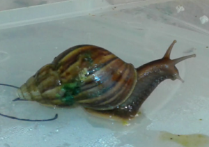
Figure 1. Giant African Snail (Lissachatina fulica, formerly Achatina fulica). Image by M. Dohm.
- This next scenario may be evaluated by you for potential sources of bias. Review the list of bias listed above. A researcher wants to do a population count of feral cats on campus. Feral cats are active at night, so he decides to set up a feeding station near a light post. The researcher sits all night in a parked car yards away and watches the feeding station for visits by cats. The researcher repeats these observations over the course of a week, moving the feeding station to different campus locations each night, and reports the total number of cats seen during the week as an estimate of the population size. Be able to discuss this study in terms of potential and actual bias.
Quiz
Including the quiz on this page, a total of 65 questions among the several subchapters, a mix of true or false and multiple choice question format.
Quiz Chapter 5
Experimental design