20.12 – Phylogenetically independent contrasts
Introduction
Assumption of independence among the subjects in a study, key assumption. Cross species comparisons as tests of correlated evolution of traits has a long history in biology research (Cornwallis and Griffin 2024). Methods have transitioned from observations to rigorous, phylogenetic tree-based statistical approaches (phylogenetic comparative methods), and continue to provide important analytical tools, eg., host adaptation and cross-species transmission of Covid-19 virus (Attwood et al 2022).
Comparisons among species for the association between body size and metabolic rate, for example Kleiber’s Law, are classic cases (Fig 1, after Table 2 in Kleiber 1947). We’ll use Kleiber’s data basal metabolic rate (BMR) and body mass for a collection of species to explore two phylogenetic comparative methods, PIC and PGLS.
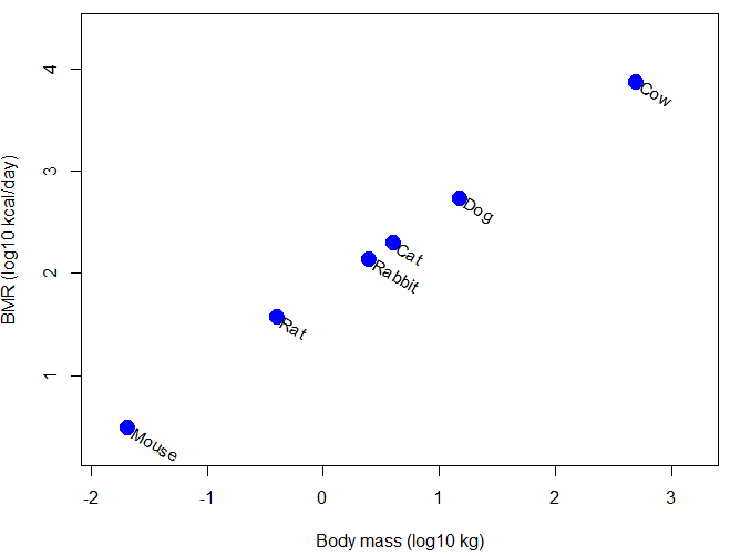
Figure 1. Scatter plot of BMR on Body Mass, log-transformed.
Typical approaches statistically, use of ANOVA or linear regression approaches. A basic assumption of ANOVA is that sampling units are independent 13.1 – ANOVA assumptions.
Prior to the 1980s, it was rarely appreciated in comparative analysis that species are not independent sample units (Harvey and Pagel 1991); evolution produced nested hierarchical relationships among the species. We recognize this with phylogenies (Felsenstein 1985, Harvey and Pagel 1991, Martins 1996, Garland et al 2005). Mice and rats share more recent common ancestor, and cattle and pigs share more recent common ancestor, than do mice and cattle, for example. Felsenstein (1985, 1988), largely credited for making the argument that Type I error likely if phylogeny ignored, and, importantly, provided an algorithm, Phylogenetic Independent Contrasts, PIC, which provided a simple way to correct for phylogenetic nonindependence. Felsentein’s landmark 1985 paper has been cited more than ten thousand times (Feb 2024).
Logic of PIC
Treating comparative data, eg, species, as a collection of independent samples implies that the evolutionary history was a spontaneous burst, or star-like phylogeny — an unresolved phylogenetic tree with branches radiating from a single ancestral node (Fig 2).
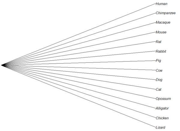
Figure 2. Star tree phylogeny (same image shown Figure 5, 20.11 – Plot a Newick tree).
But what nature provides is nonindependence (Fig 3, for more about star phylogeny in PIC see discussion in Garland et al 2005), Darwin’s “groups under groups,” or a nested hiearchy. Species are not independent units and phylogenetic history should be accounted for during statistical analysis.
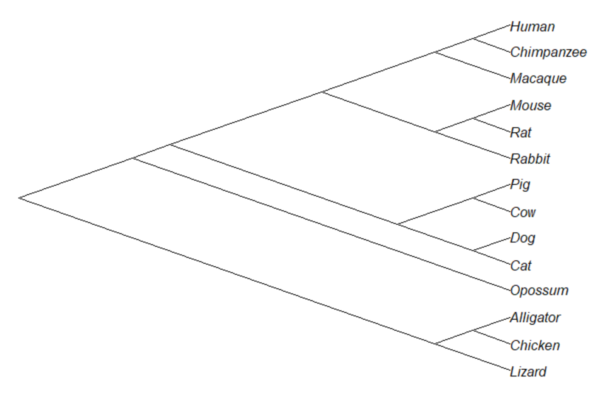
Figure 3. A cladogram for same species, showing the hierarchical, nested relationships among taxa, what nature actually provides (same image shown Figure 2, 20.11 – Plot a Newick tree).
Let’s revisit Figure 1. What do the points look like if we line up the known phylogeny for Kleiber’s six species against the plotted data? That gives us Figure 4.
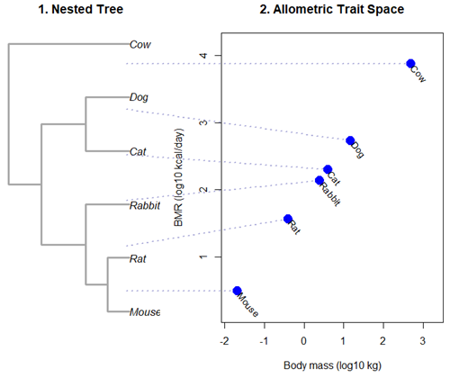
Figure 4. Kleiber’s Law and the confounding effect of shared ancestry.
Dashed connecting lines in Figure 4 trace each species from its tree position to its phenotypic value, demonstrating how phylogenetic clustering violates the independent data assumptions of standard OLS regression.
Begin R code for Figure 4, with remarks — code generated with Gemini AI assistance.
# 1. Reset the data frame
kleiber_data <- data.frame(
Species = c("Mouse", "Rat", "Rabbit", "Cat", "Dog", "Cow"),
Mass = c(0.021, 0.282, 2.45, 3.1, 13.4, 439.0),
BMR = c(3.38, 32.4, 134.0, 151.0, 506.0, 6135.0),
stringsAsFactors = FALSE
)
kleiber_data$log_Mass <- log10(kleiber_data$Mass)
kleiber_data$log_BMR <- log10(kleiber_data$BMR)

# 2. Build the exact matching standalone 6-species tree
library(ape)
newick_tree_6 <- "((((Mouse:10,Rat:10):10,Rabbit:20):20,(Cat:20,Dog:20):20):15,Cow:55);"
my_tree <- read.tree(text = newick_tree_6)

# 3. Setup a side-by-side 2-panel layout
layout(matrix(c(1, 2), nrow = 1), widths = c(1, 1.3))
par(mar = c(5, 4, 4, 1))

# PANEL 1: Plot the tree hierarchy
plot(my_tree, main = "1. Nested Tree",
edge.width = 3, edge.color = "darkgrey", cex = 1.1)

# FIXED COORDINATE MAP: 'ape' plots leaves bottom-to-top exactly matching the tree order
# We map the tree tip labels to simple integers 1 through 6
tree_heights <- 1:6
names(tree_heights) <- my_tree$tip.label

# PANEL 2: Plot the scatterplot
plot(kleiber_data$log_BMR ~ kleiber_data$log_Mass,
pch = 19, cex = 2, col = "blue",
xlab = "Body mass (log10 kg)", ylab = "BMR (log10 kcal/day)",
xlim = c(min(kleiber_data$log_Mass) - 0.2, max(kleiber_data$log_Mass) + 0.6),
ylim = c(min(kleiber_data$log_BMR) - 0.3, max(kleiber_data$log_BMR) + 0.3),
main = "2. Allometric Trait Space")

# Re-apply your custom 310-degree slanted text labels
text(kleiber_data$log_Mass + 0.05, kleiber_data$log_BMR - 0.03,
labels = kleiber_data$Species, srt = 310, adj = 0, cex = 0.9, col = "black")

# 4. CROSS-PANEL LINE CORRECTION: Draw lines across the margins safely
par(xpd = NA) # Tells R to ignore the borders of the active scatterplot window

# Calculate the left-hand margin boundaries based on the current plot limits
left_x_boundary <- min(kleiber_data$log_Mass) - 2.8

for(i in 1:nrow(kleiber_data)) {
sp <- kleiber_data$Species[i]

# A. Use a standardized geometric multiplier to align with Panel 1's vertical axis
# This formula maps the tree heights (1-6) into the scatterplot's Y coordinate scale
y_scale_factor <- (tree_heights[sp] - 1) / 5
y_span_range <- max(kleiber_data$log_BMR) - min(kleiber_data$log_BMR)
target_tree_y <- min(kleiber_data$log_BMR) + (y_scale_factor * y_span_range)

# B. Pull the actual coordinates of your blue dot
right_x <- kleiber_data$log_Mass[i]
right_y <- kleiber_data$log_BMR[i]

# C. Draw a clean, connecting line directly out to the dot
segments(x0 = left_x_boundary,
y0 = target_tree_y,
x1 = right_x,
y1 = right_y,
col = adjustcolor("darkblue", alpha.f = 0.3),
lty = 3, lwd = 2)
}

# Reset layout parameters back to normal
layout(1)
End R code.
Note 1. About the code for Figure 3. Ideally, we would use the function phylomorphospace (phytools package) to superimpose the nested tree and the plot of Kleiber’s data. For example, our code would look like
R code
library(phytools)
phylomorphospace(my_tree, trait_matrix,
label = "off", # Suppresses default horizontal text labels safely
xlab = "Body mass (log10 kg)",
ylab = "BMR (log10 kcal/day)",
xlim = c(min(kleiber_data$log_Mass) - 0.2, max(kleiber_data$log_Mass) + 0.6),
ylim = c(min(kleiber_data$log_BMR) - 0.3, max(kleiber_dat$log_BMR) + 0.3),
control = list(col.edge = "darkgrey", lwd = 3))
End R code.
However, the relationship is so perfect here that the tree lies flat on the regression line so we can’t see the tree for the line, hence our use of segments().
Phylogenetic Generalized Least Squares (PGLS).
However, like most innovations, PIC should not be blindly applied in all comparative analysis (eg, unreplicated evolutionary events, Uyeda et al 2018). Fundamentally, PIC is mathematically limited: it primarily handled simple two-variable correlations and required fully resolved, bifurcating evolutionary trees with known branch lengths. At about the same time, Grafen (1989) proposed that phylogenetic non-independence could be treated as a form of spatial autocorrelation — that is, near things are more related than distant things. Instead of computing data contrasts at individual tree nodes, Grafen introduced the phylogenetic regression, which used Generalized Least Squares (GLS) to alter how the regression algorithm treats the residual errors of species data. Improvements to phylogenetic regression are now collectively refered to as the Phylogenetic Generalized Least Squares (PGLS) (Rohlf 2001, Housworth et al 2004, Mazel et al 2016, Adams et al 2019).
Logic of PGLS.
In standard Ordinary Least Squares (OLS) regression, the residual error terms (ε) are assumed to be independent and identically distributed. In matrices, this error structure is represented by an identity matrix (I), where the off-diagonals are zero, implying that knowing about the trait value of a mouse reveals no information about the value for a rat or other rodent species.
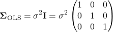
Note 2. The identity matrix  3 \times 3
 n = 3
 \sigma^{2} \times 1 = \sigma^{2}
 \sigma^{2} \times 0 = 0
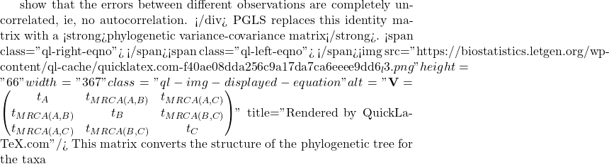
A B
 C
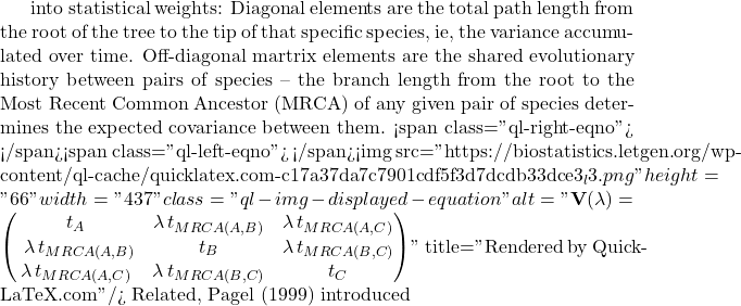
lambda Pagel’s \ \lambda
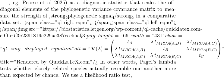
LRT \lambda

LR \chi ^{2}

\ln L_{\lambda = 0} \ln L_{\hat{\lambda}}
 \lambda
 R^{2}
 BMR = aM^{b}
 \frac{3}{4}
 n
 n – 1
 P < 0.05
 \lambda
 R^{2}$ values match identically between those two rows, while the naive OLS model stands apart due to its complete omission of tree topology.
Looking closely at the comparison of coefficients from the different models, from 0.7468 to 0.7884, it would be natural to ask, “Why go through the trouble of building a tree if the final biological answer is practically identical?” And, note that OLS and PGLS are nearly the same! The short response is only the phylogenetically correct coefficient estimates are statistically valid, and larger data sets are unlikely to reveal such agreement.
The fact that the PGLS slope (0.7674) splits the difference between the naïve OLS (0.7468) and strict PIC (0.7884) shows that Pagel’s λ converged on an intermediate value between 0 and 1. Instead of completely erasing the tree or treating it as absolute truth, PGLS multiplied the off-diagonal elements of the covariance matrix by this fractional λ value. This flattens the evolutionary branches, shrinking the expected covariance between sister taxa.
The model recognized that closely related species share some ancestral drag, but also exhibit more independent divergence than a pure random walk would predict. In contrast, the other two models represent rigid statistical boundaries:
- Naive OLS forces λ = 0, entirely ignoring the tree topology to arrive at
0.7468. - Strict PIC forces λ = 1, assuming unscaled Brownian Motion.
Because it used the full branch lengths, it shifted the trajectory heavily to 0.7884. By optimizing to an intermediate λ, PGLS strikes a perfect compromise: it protects us from the pseudoreplication of OLS while preventing the over-correction of a forced PIC.
Questions
- Mathematically, under what specific evolutionary conditions does a PGLS regression yield the exact same slope and standard error as a PIC regression?
- If your model estimates an optimized λ = 0.45, how does this physically alter the off-diagonal elements of your variance-covariance matrix compared to a standard OLS matrix?
- Why must a linear regression using Phylogenetically Independent Contrasts (PIC) be forced through the origin, omitting the standard intercept term?
- How does a PGLS matrix mathematically downweight a tight cluster of closely related species to prevent them from artificially inflating your sample size (N)?
- What happens to your Type I error rate and standard errors if you run a PGLS assuming Brownian Motion (λ = 1), but the trait actually evolved under strong stabilizing selection?
Explore on your own.
Kleiber’s data set (Table 2, 1947) contained data for humans (women) and four additional species. Redo the PIC and PGLS analysis with the updated data set. What is the effect on coefficient estimates and the standard errors with the (slightly) larger data set?
kleiber_full <- data.frame(
    Species = c("Mouse", "Rat", "Rabbit", "Macaque", "Cat", "Dog",
              "Goat", "Sheep", "Chimpanzee", "Woman", "Cow"),
# Exact body mass (W) in kilograms
    Mass = c(0.021, 0.282, 2.45, 4.20, 3.10, 13.40,
           36.00, 46.40, 38.00, 56.10, 439.00),
# Exact basal metabolic rate in kcal per 24 hours
    BMR = c(3.38, 32.7, 134.0, 207.0, 151.0, 506.0,
          826.0, 1145.0, 1090.0, 1398.0, 6135.0),
stringsAsFactors = FALSE
)
and the tree
"(((((Mouse:10,Rat:10):10,Rabbit:20):20,((Macaque:25,(Chimpanzee:6,Woman:6):19):10):10):10,(Cat:20,Dog:20):30):10,(Goat:15,Sheep:15):40,Cow:55);"
my_tree <- read.tree(text = expanded_newick)
References and suggested readings
Adams, D. C., & Collyer, M. L. (2019). Phylogenetic comparative methods and the evolution of Multivariate Phenotypes. Annual Review of Ecology, Evolution, and Systematics, 50(1):405–425.
Attwood, S. W., Hill, S. C., Aanensen, D. M., Connor, T. R., & Pybus, O. G. (2022). Phylogenetic and phylodynamic approaches to understanding and combating the early SARS-CoV-2 pandemic. Nature Reviews Genetics, 23(9), 547–562.
Blomberg, S. P., Rathnayake, S. I., & Moreau, C. M. (2020). Beyond Brownian Motion and the Ornstein-Uhlenbeck Process: Stochastic Diffusion Models for the Evolution of Quantitative Characters. American Naturalist, 195(2), 145–165.
Cornwallis, C. K., & Griffin, A. S. (2024). A guided tour of phylogenetic comparative methods for studying trait evolution. Annual Review of Ecology, Evolution, and Systematics, 55(1), 181–204.
Felsenstein, J (1985) Phylogenies and the comparative method. American Naturalist 125(1):1-15.
Felsenstein, J. (1988) Phylogenies and quantitative characters. Annual Review of Ecology and Systematics, 19, 445–471.
Garland Jr, T., Bennett, A. F., & Rezende, E. L. (2005). Phylogenetic approaches in comparative physiology. Journal of experimental Biology, 208(16), 3015-3035.
Grafen, A. (1989). The phylogenetic regression. Phil. Trans. R. Soc. London B, 326, 119-157.
Harvey, P.H. and Pagel, M.D. (1991) The Comparative Method in Evolutionary Biology. Oxford University Press, Oxford, Oxford Series in Ecology and Evolution.
Housworth, E. A., Martins, E. A. P., & Lynch, M. (2004). The phylogenetic mixed model. American Naturalist, 163, 84–96.
Kozłowski, J., & Konarzewski, M. (2004). Is West, Brown and Enquist’s model of allometric scaling mathematically correct and biologically relevant? Functional Ecology, 18(2), 283–289.
Martins, E.P. (1996) Phylogenies and the Comparative Method in Animal Behavior. Oxford University Press.
Mazel, F., Davies, T. J., Georges, D., Lavergne, S., Thuiller, W., & Peres-Neto, P. R. (2016). Improving phylogenetic regression under complex evolutionary models. Ecology, 97(2), 286–293.
Pagel, M. (1999). Inferring the historical patterns of biological evolution. Nature</i<, 401(6756), 877–884.
Paradis, E. (2012) Analysis of Phylogenetics and Evolution with R (Second Edition). New York: Springer.
Paradis, E. and Schliep, K. (2019) ape 5.0: an environment for modern phylogenetics and evolutionary analyses in R. Bioinformatics, 35, 526–528.
Pearse, W. D., Davies, T. J., & Wolkovich, E. M. (2025). How to Define, Use, and Interpret Pagel’s \ łambda \ (Lambda) in Ecology and Evolution. Global Ecology and Biogeography, 34(4), e70012.
Revell, L. J. (2012) phytools: An R package for phylogenetic comparative biology (and other things). Methods in Ecology and Evolution, 3, 217-223.
Rohlf, F. J. (2001). Comparative methods for the analysis of continuous variables: Geometric interpretations. Evolution, 55(11), 2143–2160.
Uyeda, J. C., Zenil-Ferguson, R., & Pennell, M. W. (2018). Rethinking phylogenetic comparative methods. Systematic Biology, 67(6), 1091-1109.
Zhang, J., Pei, N., & Mi, X. (2012). phylotools: Phylogenetic tools for Eco-phylogenetics. R package version 0.1, 2.
Chapter 20 contents
- Additional topics
- Area under the curve
- Peak detection
- Baseline correction
- Surveys
- Time series
- Dimensional analysis
- Estimating population size
- Diversity indexes
- Survival analysis
- Growth equations and dose response calculations
- Plot a Newick tree
- Phylogenetically independent contrasts
- How to get the distances from a distance tree
- Binary classification
- Meta-analysis