17.8 – Assumptions and model diagnostics for Simple Linear Regression
Introduction
The assumptions for all linear regression:
- Linear model is appropriate.
The data are well described (fit) by a linear model. - Independent values of Y and equal variances.
Although there can be more than one Y for any value of X, the Y‘s cannot be related to each other (that’s what we mean by independent). Since we allow for multiple Y‘s for each X, then we assume that the variances of the range of Y‘s are equal for each X value (this is similar to our ANOVA assumptions for equal variance by groups). Another term for equal variances is homoscedasticity. - Normality.
For each X value there is a normal distribution of Y‘s (think of doing the experiment over and over). - Error
The residuals (error) are normally distributed with a mean of zero.
Note the mnemonic device: Linear, Independent, Normal, Error or LINE.
Each of the four elements will be discussed below in the context of Model Diagnostics. These assumptions apply to how the model fits the data. There are other assumptions that, if violated, imply you should use a different method for estimating the parameters of the model.
Ordinary least squares makes the additional assumption about the quality of the independent variable that e that measurement of X is done without error. Measurement error is a fact of life in science, but the influence of error on regression differs if the error is associated with the dependent or independent variable. Measurement error in the dependent variable increases the dispersion of the residuals but will not affect the estimates of the coefficients; error associated with the independent variables, however, will affect estimates of the slope. In short, error in X leads to biased estimates of the slope.
The equivalent, but less restrictive practical application of this assumption is that the error in X is at least negligible compared to the measurements in the dependent variable.
Multiple regression makes one more assumption, about the relationship between the predictor variables (the X variables). The assumption is that there is no multicollinearity, a subject we will bring up next time (see Chapter 18).
Model diagnostics
We just reviewed how to evaluate the estimates of the coefficients of the model. Now we need to address a deeper meaning — how well the model explains the data. Consider a simple linear regression first. If Ho: b = 0 is not rejected — then the slope of the regression equation is taken to not differ from zero. We would conclude that if repeated samples were drawn from the population, on average, the regression equation would not fit the data well (lots of scatter) and it would not yield useful prediction.
However, recall that we assume that the fit is linear. One assumption we make in regression is that a line can, in fact, be used to describe the relationship between X and Y.
Here are two very different situations where the slope = 0.
Example 1. Linear Slope = 0, No relationship between X and Y
Example 2. Linear Slope = 0, A significant relationship between X and Y
But even if Ho: b = 0 is rejected (and we conclude that a linear relationship between X and Y is present), we still need to be concerned about the fit of the line to the data — the relationship may be more nonlinear than linear, for example. Here are two very different situations where the slope is not equal to 0.
Example 3. Linear Slope > 0, a linear relationship between X and Y
Example 4. Linear Slope > 0, curve-linear relationship between X and Y
How can you tell the difference? There are many regression diagnostic tests, many more than we can cover, but you can start with looking at the coefficient of determination (low R2 means low fit to the line), and we can look at the pattern of residuals plotted against the either the predicted values or the X variables (my favorite). The important points are:
- In linear regression, you fit a model (the slope + intercept) to the data;
- We want the usual hypothesis tests (are the coefficients different from zero?) and
- We need to check to see if the model fits the data well. Just like in our discussions of chi-square, a “perfect fit would mean that the difference between our model and the data would be zero.
Graph options
Using residual plots to diagnose regression equations
Yes, we need to test the coefficients (intercept Ho = 0; slope Ho = 0) of a regression equation, but we also must decide if a regression is an appropriate description of the data. This topic includes the use of diagnostic tests in regression. We address this question chiefly by looking at
- scatterplots of the independent (predictor) variable(s) vs. dependent (response) variable(s).
what patterns appear between X and Y? Do your eyes tell you “Line”? “Curve”? “No relation”? - coefficient of determination
closer to zero than to one? - patterns of residuals plotted against the X variables (other types of residual plots are used to, this is one of my favorites)
Our approach is to utilize graphics along with statistical tests designed to address the assumptions.
One typical choice is to see if there are patterns in the residual values plotted against the predictor variable. If the LINE assumptions hold for your data set, then the residuals should have a mean of zero with scatter about the mean. Deviations from LINE assumptions will show up in residual plots.
Here are examples of POSSIBLE outcomes:
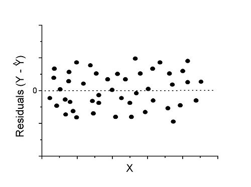
Figure 1. An ideal plot of residuals
Solution: Proceed! Assumptions of linear regression met.
Compare to plots of residuals that differ from the ideal.
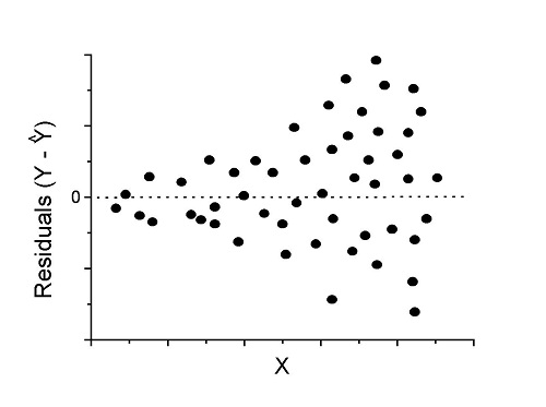
Figure 2. We have a problem. Residual plot shows a “funnel” shape — unequal variance (aka heteroscedasticity).
Solution. Try a transform like the log10-transform.
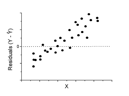
Figure 3. Problem. Residual plot shows systematic trend.
Solution. Linear model a poor fit; May be related to measurement errors for one or more predictor variables. Try adding an additional predictor variable or model the error in your general linear model.
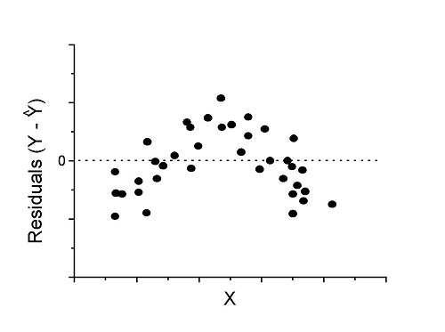
Figure 4. Problem. Residual plot shows nonlinear trend.
Solution. Transform data or use more complex model
This is a good time to mention that in statistical analyses, one often needs to do multiple rounds of analyses, involving description and plots, tests of assumptions, tests of inference. With regression, in particular, we also need to decide if our model (e.g., linear equation) is a good description of the data.
Diagnostic plot examples
Return to our example.Tadpole dataset. To obtain residual plots, Rcmdr: Models → Graphs → Basic diagnostic plots yields four graphs. Graph A is
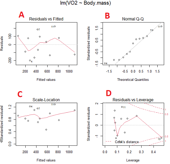
Figure 5. Basic diagnostic plots. A: residual plot; B: Q-Q plot of residuals; C: Scale-location (aka spread-location) plot; D: leverage residual plot.
In brief, we look at plots
A, the residual plot, to see if there are trends in the residuals. We are looking for a spread of points equally above and below the mean of zero. In Figure 5 we count seven points above and six points below zero so there’s no indication of a trend in the residuals vs the fitted VO2 (Y) values.
B, the Q-Q plot is used to see if normality holds. As discussed before, if our data are more or less normally distributed, then points will fall along a straight line in a Q-Q plot.
C, the Scale- or spread-location plot is used to verify equal variances of errors.
D, Leverage plot — looks to see if an outlier has leverage on the fit of the line to the data, i.e., changes the slope. Additionally, provides location of Cook’s distance measure (dashed red lines). Cook’s distance measures the effect on the regression by removing one point at a time and then fitting a line to the data. Points outside the dashed lines have influence.
A note of caution about over-thinking with these plots. R provides a red line to track the points. However, these lines are guides, not judges. We humans are generally good at detecting patterns, but with data visualization, there is the risk of seeing patterns where none exits. In particular, recognizing randomness is not easy. If anything, we may tend to see patterns where none exist, termed apophenia. So yes, by all means look at the graphs, but do so with a plan: red line more or less horizontal? Then no pattern and the regression model is a good fit to the data.
Statistical test options
After building linear models, run statistical diagnostic tests that compliment graphics approaches. Here, simply to introduce the tests, I included the Gosner factor as potential predictor — many of these numerical diagnostics are more appropriate for models with more than one predictor variable, the subject of the next chapter.
Results for the model  were:
lm(formula = VO2 ~ Body.mass + Gosner, data = frogs)

Residuals:
    Min      1Q Median    3Q    Max
-163.12 -125.53 -20.27 83.71 228.56

Coefficients:
           Estimate Std. Error t value  Pr(>|t|)
(Intercept) -595.37     239.87  -2.482 0.03487 *
Body.mass    431.20     115.15   3.745 0.00459 **
Gosner[T.II]  64.96     132.83   0.489 0.63648
---
Signif. codes: 0 '***' 0.001 '**' 0.01 '*' 0.05 '.' 0.1 ' ' 1

Residual standard error: 153.4 on 9 degrees of freedom
  (1 observation deleted due to missingness)
Multiple R-squared: 0.8047, Adjusted R-squared: 0.7613
F-statistic: 18.54 on 2 and 9 DF, p-value: 0.0006432
Question. Note the p-value for the coefficients — do we include a model with both body mass and Gosner Stage? See Chapter 18.5 – Selecting the best model
In R Commander, the diagnostic test options are available via
Rcmdr: Models → Numerical diagnostics
Variance inflation factors (VIF): used to detect multicollinearity among the predictor variables. If correlations are present among the predictor variables, then you can’t rely on the the coefficient estimates — whether predictor A causes change in the response variable depends on whether the correlated B predictor is also included in the model. If correlation between predictor A and B, the statistical effect is increased variance associated with the error of the coefficient estimates. There are VIF for each predictor variable. A VIF of one means there is no correlation between that predictor and the other predictor variables. A VIF of 10 is taken as evidence of serious multicollinearity in the model.
R code:
vif(RegModel.2)
R output
Body.mass Gosner
2.186347 2.186347

round(cov2cor(vcov(RegModel.2)), 3) # Correlations of parameter estimates
         (Intercept) Body.mass Gosner[T.II]
(Intercept)    1.000    -0.958        0.558
Body.mass     -0.958     1.000       -0.737
Gosner[T.II]   0.558    -0.737        1.000
Our interpretation
The output shows a matrix of correlations; the correlation between the two predictor variables in this model was 0.558, large per our discussions in Chapter 16.1 . Not really surprising as older tadpoles (Gosner stage II), are larger tadpoles. We’ll leave the issue of multicollinearity to Chapter 18.1.
Breusch-Pagan test for heteroscedasticity… Recall that heteroscedasticity is another name for unequal variances. This tests pertains to the residuals; we used the scale (spread) location plot (C) above. The test statistic can be calculated as  . The function call is part of the car package, which we download as part of the Rcmdr package. R Commander will pop up a menu of choices for this test. For starters, accept the defaults, enter nothing, and click OK.
R code:
library(zoo, pos=16)
library(lmtest, pos=16)
bptest(VO2 ~ Body.mass + Gosner, varformula = ~ fitted.values(RegModel.2), studentize=FALSE, data=frogs)
R output
Breusch-Pagan test

data:  VO2 ~ Body.mass + Gosner
BP = 0.0040766, df = 1, p-value = 0.9491
Our interpretation
A p-value less than 5% would be interpreted as statistically significant unequal variances among the residuals.
Durbin-Watson for autocorrelation… used to detect serial (auto)correlation among the residuals, specifically, adjacent residuals. Substantial autocorrelation can mean Type I error for one or more model coefficients. The test returns a test statistic that ranges from 0 to 4. A value at midpoint (2) suggests no autocorrelation. Default test for autocorrelation is r > 0.
R code:
dwtest(VO2 ~ Body.mass + Gosner, alternative="greater", data=frogs)
R output
Durbin-Watson test

data:  VO2 ~ Body.mass + Gosner
DW = 2.1336, p-value = 0.4657
alternative hypothesis: true autocorrelation is greater than 0
Our interpretation
The DW statistic was about 2. Per our definition, we conclude no correlations among the residuals.
RESET test for nonlinearity… The Ramsey Regression Equation Specification Error Test is used to interpret whether or not the equation is properly specified. The idea is that fit of the equation is compared against alternative equations that account for possible nonlinear dependencies among predictor and dependent variables. The test statistic follows an F distribution.
R code:
resettest(VO2 ~ Body.mass + Gosner, power=2:3, type="regressor", data=frogs)
R output
RESET test

data:  VO2 ~ Body.mass + Gosner
RESET = 0.93401, df1 = 2, df2 = 7, p-value = 0.437
Our interpretation
Also a nonsignificant test — adding a power term to account for a nonlinear trend gained no model fit benefits, p-value much greater than 5%.
Bonferroni outlier test. Reports the Bonferroni p-values for testing each observation to see if it can be considered to be a mean-shift outlier (a method for identifying potential outlier values — each value is in turn replaced with the mean of its nearest neighbors, Lehhman et al 2020). Compare to results of VIF. The objective of outlier and VIF tests is to verify that the regression model is stable, insensitive to potential leverage (outlier) values.
R code:
outlierTest(LinearModel.3)
R output
No Studentized residuals with Bonferroni p < 0.05
Largest |rstudent|:
  rstudent unadjusted p-value Bonferroni p
7 1.958858        0.085809              NA
Our interpretation
We ran the outlierTest() function on LinearModel.3 to check for influential outliers using Studentized residuals with Bonferroni correction.
The output shows “No Studentized residuals with Bonferroni p < 0.05”, which means no data points were statistically flagged as outliers after adjusting for multiple comparisons. The largest Studentized residual was 1.96 (point 7), with an unadjusted p-value of 0.086. Although this is the largest deviation from the regression line, it is not statistically significant. Therefore, we conclude that no single observation is exerting undue influence on the model fit, and we can be confident that our regression results are not driven by outliers.
Response transformation… The concept of transformations of data to improve adherence to statistical assumptions was introduced in Chapters 3.2, 13.1, and 15.
R code:
summary(powerTransform(LinearModel.3, family="bcPower"))
R output
bcPower Transformation to Normality
    Est Power Rounded Pwr Wald Lwr Bnd Wald Upr Bnd
Y1     0.9987           1       0.2755       1.7218

Likelihood ratio test that transformation parameter is equal to 0
   (log transformation)
                           LRT df      pval
LR test, lambda = (0) 7.374316  1 0.0066162

Likelihood ratio test that no transformation is needed
                                LRT df    pval
LR test, lambda = (1) 0.00001289284  1 0.99714
Our interpretation
The Box-Cox analysis suggests that the response variable for LinearModel.3 can remain on its original scale. No power transformation was needed, and any standard linear regression inference is appropriate. The estimated transformation parameter was close to one, which suggests that the original response variable did not need a transformation. The LRT tests whether a log transformation (lambda = 0) would improve normality. The significant p-value, 0.0066, for the LRT indicates that a log transformation would not be the best choice, consistent with lambda ≈ 1. And last, the very high p-value, 0.99714, confirms that no transformation is necessary; the model residuals were close to normal.
Questions
- Write up three learning outcomes for this page. Hint: Point your favorite generative AI to this page and ask for help.
- Referring to Figures 1 – 4 on this page, which plot best suggests a regression line fits the data?
- Return to the electoral college data set and your linear models of Electoral vs. POP_2010 and POP_2019. Obtain the four basic diagnostic plots and comment on the fit of the regression line to the electoral college data.
- residual plot
- Q-Q plot
- Scale-location plot
- Leverage plot
- With respect to your answers in question 2, how well does the electoral college system reflect the principle of one person one vote?
Quiz Chapter 17.8
Assumptions and model diagnostics for Simple Linear Regression
Chapter 17 contents
- Introduction
- Simple Linear Regression
- Relationship between the slope and the correlation
- Estimation of linear regression coefficients
- OLS, RMA, and smoothing functions
- Testing regression coefficients
- Regression model fit
- Assumptions and model diagnostics for Simple Linear Regression
- References and suggested readings (Ch17 & 18)
16.2 – Causation and Partial correlation
Introduction
Science driven by statistical inference and model building is largely motivated by the the drive to identify pathways of cause and effect linking events and phenomena observed all around us. (We first defined cause and effect in Chapter 2.4) The history of philosophy, from the works of Ancient Greece, China, Middle East and so on is rich in the language of cause and effect. From these traditions we have a number of ways to think of cause and effect, but for us it will be enough to review the logical distinction among three kinds of cause-effect associations:
- Necessary cause
- Sufficient cause
- Contributory cause
Here’s how the logic works. If A is a necessary cause of B, then the mere fact that B is present implies that A must also be present. However, that the presence of A does not imply that B will occur. If A is a sufficient cause of B, then the presence of A necessarily implies the presence of B. However, another cause C may alternatively cause B. Enter the contributory or related cause: A cause may be contributory if the presumed cause A (1) occurs before the effect B, and (2) changing A also changes B. A contributory cause does not need to be necessary nor must it be sufficient; contributory causes play a role in cause and effect.
Thus, following this long tradition of thinking about causality we have the mantra, “Correlation does not imply causation.” The exact phrase was written as early as emphasized by Karl Pearson who invented the statistic back in the late 1800s. This well-worn slogan deserves to be on T-shirts and bumper stickers*, and perhaps to be viewed as the single most important concept you can take from a course in philosophy/statistics. But in practice, we will always be tempted to stray from this guidance. The developments in genome-wide-association studies, or GWAS, are designed to look for correlations, as evidenced by statistical linkage analysis, between variation at one DNA base pair and presence/absence of disease or condition in humans and animal models. These are costly studies to do and in the end, the results are just that, evidence of associations (correlations), not proof of genetic cause and effect. We are less likely to be swayed by a correlation that is weak, but what about correlations that are large, even close to one? Is not the implication of high, statistically significant correlation evidence of causation? No, necessary, but not sufficient.
Note 1. A helpful review on causation in epidemiology is available from Parascandola and Weed (2001); see also Kleinberg and Hripcsak (2011). For more on “correlation does not imply causation”, try the Wikipedia entry. Obviously, researchers who engage in genome wide association studies are aware of these issues: see for example discussion by Hu et al (2018) on causal inference and GWAS.
Causal inference (Pearl 2009; Pearl and Mackenzie 2018), in brief, employs a model to explain the association between dependent and multiple, likely interrelated candidate causal variable, which is then subject to testing — is the model stable when the predictor variables are manipulated, when additional connections are considered (eg, predictor variable 1 covaries with one or more other predictor variables in the model). Wright’s path analysis, now included as one approach to Structural Equation Modeling, is used to relate equations (models) of variation in observed variables attributed to direct and indirect effects from predictor variables.
* And yes, a quick Google search reveals lots of bumper stickers and T-shirts available with the causation  sentiment.
Spurious correlations
Correlation estimates should be viewed as hypotheses in the scientific sense of the meaning of hypotheses for putative cause-effect pairings. To drive the point home, explore the web site “Spurious Correlations” at https://www.tylervigen.com/spurious-correlations , which allows you to generate X-Y plots and estimate correlations among many different variables. Some of my favorite correlations from “Spurious Correlations” include (Table 1):
Table 1. Spurious correlations, https://www.tylervigen.com/spurious-correlations
| First variable | Second variable | Correlation |
| Divorce rate in Maine, USA | Per capita USA consumption of margarine | +0.993 |
| Honey producing bee colonies USA | Juvenile arrests for marijuana possession | -0.933 |
| Per capita USA consumption of mozzarella cheese | Civil engineering PhD awarded USA | +0.959 |
| Total number of ABA lawyers USA | Cost of red delicious apples | +0.879 |
These are some pretty strong correlations (cf. effect size discussion, Ch11.4 and 16.1), about as close to +1 as you can get. But really, do you think the amount of cheese that is consumed in the USA has anything to do with the number of PhD degrees awarded in engineering or that apple prices are largely set by the number of lawyers in the USA? Cause and effect implies there must also be some plausible mechanism, not just a strong correlation.
But that does NOT ALSO mean that a high correlation is meaningless. The primary reason a correlation cannot tell about causation is because of the problem (potentially) of an UNMEASURED variable (a confounding variable) being the real driving force (Fig 1).
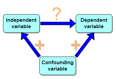
Figure 1. Unmeasured confounding variables influence association between independent and dependent variables, the characters or traits we are interested in.
Here’s a plot of running times for the best, fastest men and women runners for the 100-meter sprint. Running times over 100 meters of top athletes since the 1920s. The data are collated for you and presented at end of this page (scroll or click here).
Here’s a scatterplot (Fig 2).
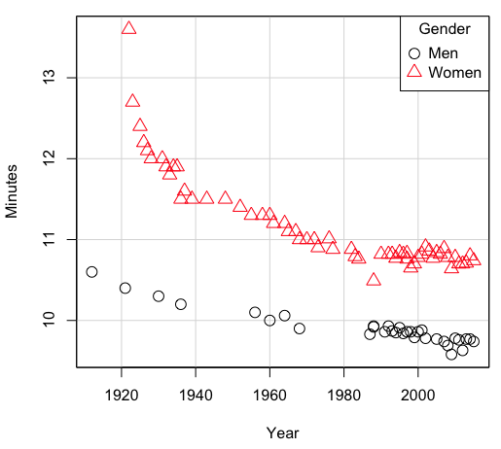
Figure 2. Running times over 100 meters of top athletes since the 1920s.
There’s clearly a negative correlation between years and running times. Is the rate of improvement in running times the same for men and women? Is the improvement linear? What, if any, are the possible confounding variables? Height? weight? Biomechanical differences? Society? Training? Genetics? … Performance enhancing drugs…?
If we measure potential confounding factors, we may be able to determine the strength of correlation between two variables that share variation with a third variable.
The partial correlation
There are several ways to work this problem. The partial correlation is a useful way to handle this problem, i.e., where a measured third variable is positively correlated with the two variable you are interested in.

Without formal mathematical proof presented, r12.3 is the correlation between variables 1 and 2 INDEPENDENT of any covariation with variable 3.
For our running data set, we have the correlation between women’s time for 100m over 9 decades, (r13 = -0.876), between men’s time for 100m over 9 decades (r23 = -0.952), and finally, the correlation we’re interested in, whether men’s and women’s times are correlated (r12 = +0.71). When we use the partial correlation, however, I get r12.3 = -0.819… much less than 0 and significantly different from zero. In other words, men’s and women’s times are not positively correlated independent of the correlation both share with the passage of time (decades)! The interpretation is that men are getting faster at a rate faster than women.
In conclusion, keep your head about you when you are doing analyses. You may not have the skills or knowledge to handle some problems (partial correlation), but you can think simply — why are two variables correlated? One causes the other to increase (or decrease) OR the two are both correlated with another variable.
Testing the partial correlation
Like our simple correlation, the partial correlation may be tested by a t-test, although modified to account for the number of pairwise correlations (Wetzels and Wagenmakers 2012). The equation for the t test statistic is now
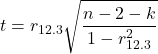
with k equal to the number of pairwise correlations and n – 2 – k degrees of freedom.
Examples
Lead exposure and low birth weigh. The data set is numbers of low birth weight births (< 2,500 g regardless of gestational age) and numbers of children with high levels of lead (10 or more micrograms of lead in a deciliter of blood) measured from their blood. Data used for 42 cities and towns of Rhode Island, United States of America (data at end of this page, scroll or click here to access the data).
A scatterplot of number of children with high lead is shown below (Fig 3).
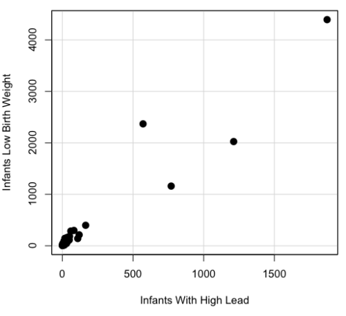
Figure 3. Scatterplot birth weight by lead exposure.
The product moment correlation was r = 0.961, t = 21.862, df = 40, p < 2.2e-16. So, at first blush looking at the scatterplot and the correlation coefficient, we conclude that there is a significant relationship between lead and low birth weight, right?
However, by the description of the data you should recall that counts were reported, not rates (eg, per 100,000 people). Clearly, population size varies among the cities and towns of Rhode Island. West Greenwich had 5085 people whereas Providence had 173,618. We should suspect that there is also a positive correlation between number of children born with low birth weight and numbers of children with high levels of lead. Indeed there are.
Correlation between Low Birth Weight and Population, r = 0.982
Correlation between High Lead levels and Population, r = 0.891
The question becomes, after removing the covariation with population size is there a linear association between high lead and low birth weight? One option is to calculate the partial correlation. To get partial correlations in Rcmdr, select
Statistics → Summaries → Correlation matrix
then select “partial” and select all three variables (select + Ctrl key; (Windows or macOS) (Fig 4).
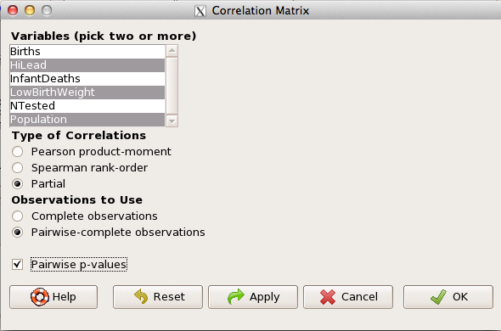
Figure 4. Screenshot Rcmdr partial correlation menu
Results are shown below.
partial.cor(leadBirthWeight[,c("HiLead","LowBirthWeight","Population")], tests=TRUE, use="complete")

Partial correlations:
                 HiLead LowBirthWeight Population
HiLead          0.00000        0.99181   -0.97804
LowBirthWeight  0.99181        0.00000    0.99616
Population     -0.97804        0.99616    0.00000
Thus, after removing the covariation we conclude there is indeed a strong correlation between lead and low birth weights.
Note 2. Some verbiage about correlation tables (matrices). The matrix is symmetric and the information is repeated. I highlighted the diagonal in green. The upper triangle (red) is identical to the lower triangle (blue). When you publish such matrices, don’t publish both the upper and lower triangles; it’s also not necessary to publish the on-diagonal numbers, which are generally not of interest. Thus, the publishable matrix would be
Partial correlations:
                LowBirthWeight Population
HiLead                 0.99181   -0.97804
LowBirthWeight                    0.99616
Another example
Do Democrats prefer cats? The question I was interested in, Do liberals really prefer cats, was inspired by a Time magazine 18 February 2014 article. I collated data on a separate but related question: Do states with more registered Democrats have more cat owners? The data set was compiled from three sources: 2010 USA Census, a 2011 Gallup poll about religious preferences, and from a data book on survey results of USA pet owners (data at end of this page, scroll or click here to access the data).
Note 3: This type of data set involves questions about groups, not individuals. We have access to aggregate statistics for groups (city, county, state, region), but not individuals. Thus, our conclusions are about groups and cannot be used to predict individual behavior, eg, knowing a person votes Green Party does not mean they necessarily share their home with a cat). See ecological fallacy.
This data set also demonstrates use of transformations of the data to improve fit of the data to statistical assumptions (normality, homoscedacity).
The variables, and their definitions, were:
ASDEMS = DEMOCRATS. Democrat advantage: the difference in registered Democrats compared to registered Republicans as a percentage; to improve the distribution qualities the arcsine transform was applied..
ASRELIG = RELIGION. Percent Religious from a Gallup poll who reported that Religion was “Very Important” to them. Also arcsine-transformed to improve normality and homoescedasticity (there you go, throwing $3 words around 🤠 ).
LGCAT = Number of pet cats, log10-transformed, estimated for USA states by survey, except Alaska and Hawaiʻi (not included in the survey by the American Veterinary Association).
LGDOG = Estimated number of pet dogs, log10-transformed for states, except Alaska and Hawaiʻi (not included in the survey by the American Veterinary Association).
LGIPC = Per capita income, log10-transformed.
LGPOP = Population size of each state, log10 transformed.
As always, begin with data exploration. All of the variables were right-skewed, so I applied data transformation functions as appropriate: log10 for the quantitative data and arc sine transform for the frequency variables. Because Democrat Advantage and Percent Religious variables were in percentages, the values were first divided by 100 to make frequencies, then the R function asin() was applied. All analyses were conducted on the transformed data, therefore conclusions apply to the transformed data.
Note 4: As we’ve discussed before, to relate the results to the original scales, back transformations would need to be run on any predictions. Back transformation for log10 would be power of ten; for the arcsine-transform the inverse of the arcsine would be used.
A scatter plot matrix (KMggplo2) plus histograms of the variables along the diagonals shows the results of the transforms and hints at the associations among the variables. A graphic like this one is called a trellis plot; a layout of smaller plots in a grid with the same (preferred) or at least similar axes. Trellis plots (Fig 5) are useful for finding the structure and patterns in complex data. Scanning across a row shows relationships between one variable with all of the others. For example, the first row Y-axis is for the ASDEMS variable; from left to right along the row we have, after the histogram, what look to be weak associations between ASDEMS and ASRELIG, LGCAT, LGDOG, and LGDOG.
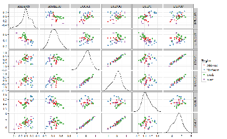
Figure 5. Trellis plot, correlations among variables.
A matrix of partial correlations was produced from the Rcmdr correlation call. Thus, to pick just one partial correlation, the association between DEMOCRATS and RELIGION (reported as “very important”) is negative (r = -0.45) and from the second matrix we retrieve the approximate P-value, unadjusted for the multiple comparisons problem, of p = 0.0024. We quickly move past this matrix to the adjusted P-values and confirm that this particular correlation is statistically significant even after correcting for multiple comparisons. Thus, there is a moderately strong negative correlation between those who reported that religion was very important to them and the difference between registered Democrats and Republicans in the 48 states. Because it is a partial correlation, we can conclude that this correlation is independent of all of the other included variables.
And what about our original question: Do Democrats prefer cats over dogs? The partial correlation after adjusting for all of the other correlated variables is small (r = 0.05) and not statistically different from zero (P-value greater than 5%).
Are there any interesting associations involving pet ownership in this data set? See if you can find it (hint: the correlation you are looking for is also in red).
Partial correlations:
         ASDEMS  ASRELIG LGCAT   LGDOG   LGIPC   LGPOP
ASDEMS   0.0000 -0.4460  0.0487  0.0605  0.1231 -0.0044
ASRELIG -0.4460  0.0000 -0.2291 -0.0132 -0.4685  0.2659
LGCAT    0.0487 -0.2291  0.0000  0.2225 -0.1451  0.6348
LGDOG    0.0605 -0.0132  0.2225  0.0000 -0.6299  0.5953
LGIPC    0.1231 -0.4685 -0.1451 -0.6299  0.0000  0.6270
LGPOP   -0.0044  0.2659  0.6348  0.5953  0.6270  0.0000
Raw P-values, Pairwise two-sided p-values:
         ASDEMS ASRELIG  LGCAT   LGDOG   LGIPC   LGPOP
ASDEMS           0.0024  0.7534  0.6965  0.4259  0.9772
ASRELIG  0.0024          0.1347  0.9325  0.0013  0.0810
LGCAT    0.7534  0.1347          0.1465  0.3473  <.0001
LGDOG    0.6965  0.9325  0.1465          <.0001  <.0001
LGIPC    0.4259  0.0013  0.3473  <.0001          <.0001
LGPOP    0.9772  0.0810  <.0001  <.0001  <.0001
Adjusted P-values, Holm’s method (Benjamini and Hochberg 1995)
         ASDEMS ASRELIG  LGCAT   LGDOG   LGIPC   LGPOP
ASDEMS           0.0241  1.0000  1.0000  1.0000  1.0000
ASRELIG  0.0241          1.0000  1.0000  0.0147  0.7293
LGCAT    1.0000  1.0000          1.0000  1.0000  <.0001
LGDOG    1.0000  1.0000  1.0000          <.0001  0.0002
LGIPC    1.0000  0.0147  1.0000  <.0001          <.0001
LGPOP    1.0000  0.7293  <.0001  0.0002  <.0001
A graph (Fig 6) to summarize the partial correlations: green lines indicate positive correlation, red lines show negative correlations; Strength of association indicated by the line thickness, with thicker lines corresponding to greater correlation.
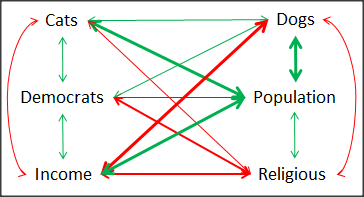
Figure 6. Causal paths among variables.
As you can see, partial correlation analysis is good for a few variables, but as the numbers increase it is difficult to make heads or tails out of the analysis. Better methods for working with these highly correlated data in what we call multivariate data analysis, for example Structural Equation Modeling or Path Analysis.
Questions
- Write up three learning outcomes for this page. Hint: Point your favorite generative AI to this page and ask for help.
- Spurious correlations can be challenging to recognize, and, sometimes, they become part of a challenge to medicine to explain away. A classic spurious correlation is the correlation between rates of MMR vaccination and autism prevalence. Here’s a table of numbers for you
| Year | Herb Supplement Revenue, millions $ | Fertility rate per 1000 births, women age 35 and older+ | MMR per 100K children age 0 -5 | UFC revenue, millions $ | Autism Prevalence per 1000 |
|---|---|---|---|---|---|
| 2000 | 4225 | 47.7 | 179 | 6.7 | |
| 2001 | 4361 | 48.6 | 183 | 4.5 | |
| 2002 | 4275 | 49.9 | 190 | 8.7 | 6.6 |
| 2003 | 4146 | 52.6 | 196 | 7.5 | |
| 2004 | 4288 | 54.5 | 199 | 14.3 | 8 |
| 2005 | 4378 | 55.5 | 197 | 48.3 | |
| 2006 | 4558 | 56.9 | 198 | 180 | 9 |
| 2007 | 4756 | 57.6 | 204 | 226 | |
| 2008 | 4800 | 56.7 | 202 | 275 | 11.3 |
| 2009 | 5037 | 56.1 | 201 | 336 | |
| 2010 | 5049 | 56.1 | 209 | 441 | 14.4 |
| 2011 | 5302 | 57.5 | 212 | 437 | |
| 2012 | 5593 | 58.7 | 216 | 446 | 14.5 |
| 2013 | 6033 | 59.7 | 220 | 516 | |
| 2014 | 6441 | 61.6 | 224 | 450 | 16.8 |
| 2015 | 6922 | 62.8 | 222 | 609 | |
| 2016 | 7452 | 64.1 | 219 | 666 | 18.5 |
| 2017 | 8085 | 63.9 | 213 | 735 | |
| 2018 | 65.3 | 220 | 800 | 25 |
- Make scatterplots of autism prevalence vs
- Herb supplement revenue
- Fertility rate
- MMR vaccination
- UFC revenue
- Calculate and test correlations between autism prevalence vs
- Herb supplement revenue
- Fertility rate
- MMR vaccination
- UFC revenue
- Interpret the correlations — is there any clear case for autism vs MMR?
- What additional information is missing from Table 2? Add that missing variable and calculate partial correlations for autism prevalence vs
- Herb supplement revenue
- Fertility rate
- MMR vaccination
- UFC revenue
- Do a little research: What are some reasons for increase in autism prevalence? What is the consensus view about MMR vaccine and risk of autism?
Quiz Chapter 16.2
Causation and Partial correlation
Data sets
Data used in this page, 100 meter running times since 1900.
| Year | Men | Women |
|---|---|---|
| 1912 | 10.6 | |
| 1913 | ||
| 1914 | ||
| 1915 | ||
| 1916 | ||
| 1917 | ||
| 1918 | ||
| 1919 | ||
| 1920 | ||
| 1921 | 10.4 | |
| 1922 | 13.6 | |
| 1923 | 12.7 | |
| 1924 | ||
| 1925 | 12.4 | |
| 1926 | 12.2 | |
| 1927 | 12.1 | |
| 1928 | 12 | |
| 1929 | ||
| 1930 | 10.3 | |
| 1931 | 12 | |
| 1932 | 11.9 | |
| 1933 | 11.8 | |
| 1934 | 11.9 | |
| 1935 | 11.9 | |
| 1936 | 10.2 | 11.5 |
| 1937 | 11.6 | |
| 1938 | ||
| 1939 | 11.5 | |
| 1940 | ||
| 1941 | ||
| 1942 | ||
| 1943 | 11.5 | |
| 1944 | ||
| 1945 | ||
| 1946 | ||
| 1947 | ||
| 1948 | 11.5 | |
| 1949 | ||
| 1950 | ||
| 1951 | ||
| 1952 | 11.4 | |
| 1953 | ||
| 1954 | ||
| 1955 | 11.3 | |
| 1956 | 10.1 | |
| 1957 | ||
| 1958 | 11.3 | |
| 1959 | ||
| 1960 | 10 | 11.3 |
| 1961 | 11.2 | |
| 1962 | ||
| 1963 | ||
| 1964 | 10.06 | 11.2 |
| 1965 | 11.1 | |
| 1966 | ||
| 1967 | 11.1 | |
| 1968 | 9.9 | 11 |
| 1969 | ||
| 1970 | 11 | |
| 1972 | 10.07 | 11 |
| 1973 | 10.15 | 10.9 |
| 1976 | 10.06 | 11.01 |
| 1977 | 9.98 | 10.88 |
| 1978 | 10.07 | 10.94 |
| 1979 | 10.01 | 10.97 |
| 1980 | 10.02 | 10.93 |
| 1981 | 10 | 10.9 |
| 1982 | 10 | 10.88 |
| 1983 | 9.93 | 10.79 |
| 1984 | 9.96 | 10.76 |
| 1987 | 9.83 | 10.86 |
| 1988 | 9.92 | 10.49 |
| 1989 | 9.94 | 10.78 |
| 1990 | 9.96 | 10.82 |
| 1991 | 9.86 | 10.79 |
| 1992 | 9.93 | 10.82 |
| 1993 | 9.87 | 10.82 |
| 1994 | 9.85 | 10.77 |
| 1995 | 9.91 | 10.84 |
| 1996 | 9.84 | 10.82 |
| 1997 | 9.86 | 10.76 |
| 1998 | 9.86 | 10.65 |
| 1999 | 9.79 | 10.7 |
| 2000 | 9.86 | 10.78 |
| 2001 | 9.88 | 10.82 |
| 2002 | 9.78 | 10.91 |
| 2003 | 9.93 | 10.86 |
| 2004 | 9.85 | 10.77 |
| 2005 | 9.77 | 10.84 |
| 2006 | 9.77 | 10.82 |
| 2007 | 9.74 | 10.89 |
| 2008 | 9.69 | 10.78 |
| 2009 | 9.58 | 10.64 |
| 2010 | 9.78 | 10.78 |
| 2011 | 9.76 | 10.7 |
| 2012 | 9.63 | 10.7 |
| 2013 | 9.77 | 10.71 |
| 2014 | 9.77 | 10.8 |
| 2015 | 9.74 | 10.74 |
| 2016 | 9.8 | 10.7 |
| 2017 | 9.82 | 10.71 |
| 2018 | 9.79 | 10.85 |
| 2019 | 9.76 | 10.71 |
| 2020 | 9.86 | 10.85 |
| 2021 | 9.77 | 10.54 |
| 2022 | 9.76 | 10.62 |
| 2023 | 9.83 | 10.65 |
| 2024 | 9.77 | 10.72 |
Data used in this page, birth weight by lead exposure
| CityTown | Core | Population | NTested | HiLead | Births | LowBirthWeight | InfantDeaths |
|---|---|---|---|---|---|---|---|
| Barrington | n | 16819 | 237 | 13 | 785 | 54 | 1 |
| Bristol | n | 22649 | 308 | 24 | 1180 | 77 | 5 |
| Burrillville | n | 15796 | 177 | 29 | 824 | 44 | 8 |
| Central Falls | y | 18928 | 416 | 109 | 1641 | 141 | 11 |
| Charlestown | n | 7859 | 93 | 7 | 408 | 22 | 1 |
| Coventry | n | 33668 | 387 | 20 | 1946 | 111 | 7 |
| Cranston | n | 79269 | 891 | 82 | 4203 | 298 | 20 |
| Cumberland | n | 31840 | 381 | 16 | 1669 | 98 | 8 |
| East Greenwich | n | 12948 | 158 | 3 | 598 | 41 | 3 |
| East Providence | n | 48688 | 583 | 51 | 2688 | 183 | 11 |
| Exeter | n | 6045 | 73 | 2 | 362 | 6 | 1 |
| Foster | n | 4274 | 55 | 1 | 208 | 9 | 0 |
| Glocester | n | 9948 | 80 | 3 | 508 | 32 | 5 |
| Hopkintown | n | 7836 | 82 | 5 | 484 | 34 | 3 |
| Jamestown | n | 5622 | 51 | 14 | 215 | 13 | 0 |
| Johnston | n | 28195 | 333 | 15 | 1582 | 102 | 6 |
| Lincoln | n | 20898 | 238 | 20 | 962 | 52 | 4 |
| Little Compton | n | 3593 | 48 | 3 | 134 | 7 | 0 |
| Middletown | n | 17334 | 204 | 12 | 1147 | 52 | 7 |
| Narragansett | n | 16361 | 173 | 10 | 728 | 42 | 3 |
| Newport | y | 26475 | 356 | 49 | 1713 | 113 | 7 |
| New Shoreham | n | 1010 | 11 | 0 | 69 | 4 | 1 |
| North Kingstown | n | 26326 | 378 | 20 | 1486 | 76 | 7 |
| North Providence | n | 32411 | 311 | 18 | 1679 | 145 | 13 |
| North Smithfield | n | 10618 | 106 | 5 | 472 | 37 | 3 |
| Pawtucket | y | 72958 | 1125 | 165 | 5086 | 398 | 36 |
| Portsmouth | n | 17149 | 206 | 9 | 940 | 41 | 6 |
| Providence | y | 173618 | 3082 | 770 | 13439 | 1160 | 128 |
| Richmond | n | 7222 | 102 | 6 | 480 | 19 | 2 |
| Scituate | n | 10324 | 133 | 6 | 508 | 39 | 2 |
| Smithfield | n | 20613 | 211 | 5 | 865 | 40 | 4 |
| South Kingstown | n | 27921 | 379 | 35 | 1330 | 72 | 10 |
| Tiverton | n | 15260 | 174 | 14 | 516 | 29 | 3 |
| Warren | n | 11360 | 134 | 17 | 604 | 42 | 1 |
| Warwick | n | 85808 | 973 | 60 | 4671 | 286 | 26 |
| Westerly | n | 22966 | 140 | 11 | 1431 | 85 | 7 |
| West Greenwich | n | 5085 | 68 | 1 | 316 | 15 | 0 |
| West Warwick | n | 29581 | 426 | 34 | 2058 | 162 | 17 |
| Woonsoket | y | 43224 | 794 | 119 | 2872 | 213 | 22 |
Data in this page, Do Democrats prefer cats?
Chapter 16 contents
- Introduction
- Product moment correlation
- Causation and Partial correlation
- Data aggregation and correlation
- Spearman and other correlations
- Instrument reliability and validity
- Similarity and Distance
- References and suggested readings
13.4 – Tests for Equal Variances
Introduction
In order to carry out statistical tests correctly, we must test our data first to see if our sample conforms to the assumptions of the statistical test. If our data do not meet these assumptions, then inferences drawn may be incorrect. How far off our inferences may be depends on a number of factors, but mostly it depends on how far from the expectations our data are.
One assumption we make with parametric tests involving ratio scale data is that the data could be from a normally distributed population. The other key assumption introduced, but not described in detail for the two-sample t-test, was that the variability in the two groups must be the same, ie, homoscedasticity. Thus, in order to carry out the independent sample t-test, we must assume that the variances are equal.
There are two general reasons we may want to concern ourselves with a test for the differences between two variances
- The t-test (and other tests like one-way ANOVA) requires that the two samples compared have the same variances. If the Variances are Not Equal we need to perform a modified t-test (see Welch’s formula).
- We may also be interested in the differences between the variances in two populations.
Example 1: In genetics we might be interested in the difference between the variability of response of inbred lines (little genetic variation but environmental variation) versus an outbred populations (lots of genetic and environmental variation).
Example 2: Environmental stress can cause organisms to have developmental instability. This might cause organisms to be more variable in morphology or the two sides (right & left) of an organism may develop non-symmetrically. Therefore, polluted environments might cause organisms to have greater variability compared to non-polluted environments.
The first way to test the variances is to use the F test. This works for two groups.

For more than two groups, we’ll use different tests (eg, Bartlett’s test, Levene’s test).
Remember that the formula for the sample variance is
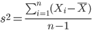
The Null Hypothesis is that the two samples have the same variances:

The Alternative Hypothesis is that the two samples do not have the same variances:

Note: I prefer to evaluate this as a one-tailed test: identify the larger of the two variances and take that as the numerator Then, the null hypothesis is that

and therefore, the alternative hypothesis is that (ie, a one-tailed test).

Another way to state equal variance test is that we are testing for homogeneity of variances. You may run across the term homoscedasticity; it is the same thing, just a different three dollar word for “equal variances.”
Stated yet another way, if we reject the null hypothesis, then the variances are unequal or show heterogeneity. An additional and equivalent $3 word for inequality of variances is called heteroscedasticity.
More about the F-test
For the F-test, the null hypothesis is that the variances are equal. This means that the “expected” F value will be one: F = 1.0. (The F-distribution differs from t-distribution because it requires 2 values for DF, and ranges from 1 to infinity for every possible combination of v1 and v2).
To evaluate the null hypothesis we need the degrees of freedom. For the F test we need two different degrees of freedom, one set for each group): from Table 2, Appendix – F distribution, look up 5% Type I error line in this table because we make it one tailed.
I need the F-test statistic at 
Examples of difference between two variances, Table 1.
Sample 1: Aggressiveness of Inbred Mice (number of bites in 30 minutes)
Sample 2: Aggressiveness of Outbred Mice (number of bites in 30 minutes)
Table 1. Aggression by inbred and outbred mice.
| Sample 1
Aggressiveness of Inbred Mice |
Sample 2
Aggressiveness of Outbred Mice |
| 3 | 4 |
| 5 | 10 |
| 4 | 4 |
| 3 | 7 |
| 4 | 7 |
| 5 | 10 |
| 4 = mean | 7 = mean |
- Identify the null and alternative hypotheses
- Calculate Variances
- Calculate F-test
- The “test statistic” for this hypothesis test was F = 7.2 / 0.8 = 9.0
- Determine Critical Value of the F table (Table 2, Appendix – F distribution)
Example of how to find the critical values of the F distribution for  and numerator
 and denominator
 .
Table 2. Portion of F distribution, see Appendix – F distribution.
| α = 0.05 | v1 | ||||||||
| 1 | 2 | 3 | 4 | 5 | 6 | 7 | 8 | ||
| v2 | 1 | 230 | |||||||
| 2 | 19.3 | ||||||||
| 3 | 9.01 | ||||||||
| 4 | 6.26 | ||||||||
| 5 | 6.61 | 5.79 | 5.41 | 5.19 | 5.05 | 4.95 | 4.88 | 4.82 | |
| 6 | |||||||||
Or, instead of using tables, use R
Rcmdr: Distributions → F distribution → F probabilities
and enter the numbers as shown below (Fig 1).
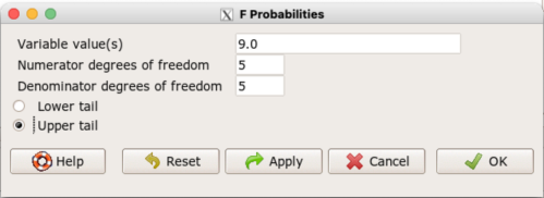
Figure 1. Screenshot R Commander F distribution probabilities.
This will return the p-value, and you would interpret this against your Type I error rate of 5% as you do for other tests.
From Table 2, Appendix – F distribution we find 
And the p-value = 0.015
pf(c(9), df1=5, df2=5, lower.tail=FALSE)
[1] 0.01537472
Question: Reject or Accept null hypothesis?
Question: What is the biological interpretation or conclusion from this result?
R code
Rather than play around with the tables of critical values, which are awkward and old-school (and I am showing you these stats tables so that you get a feel for the process, not so you’d actually use them in real practice), use Rcmdr to generate the F test and therefore return the F distribution probability value. As you may expect, R provides a number of options for testing the equal variances assumption, including the F test. The F test is limited to only two groups and, because it is a parametric test, it also makes the assumption of normality, so the F test should not be viewed as necessarily the best test for the equal variances assumption among groups. We present it here because it is a logical test to understand and because of its relevance to the Mean Square ratios in the ANOVA procedures.
So, without further justification, here is the presentation on how to get the F test in Rcmdr. At the end of this section I present a better procedure than the F test for evaluating the equal variance assumption called the Levene test.
Return to the bite data in the table above and enter the data into an R data frame. Note that the data in the table above are unstacked; R expects the data to be stacked, so either create a stacked worksheet and transcribe the data appropriately into the cells of the worksheet, or, go ahead and enter the values into two separate columns then use the Stack variables in active data set… command from the Data menu in Rcmdr.
Then, proceed to perform the F test.
Rcmdr: Statistics → Variances → Two variances F-test…
The first context menu popup is where you enter the variables (Fig 2).
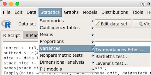
Figure 2. Screenshot data options R Commander F test
Because there are only two variables in the data set and because Strain contains the text labels of inbred or outbred whereas the other variable is numeric data type, R will correctly select the variables for you by default. Select the “Options” tab to set the parameters of the F test (Fig 3).
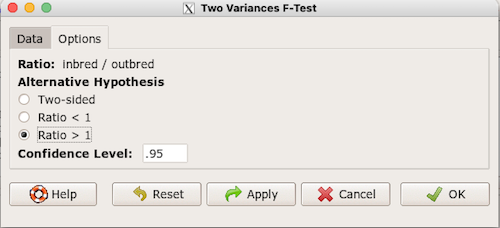
Figure 3. Screenshot menu options R Commander F test.
When you are finished setting the alternative hypothesis and confidence levels, proceed with the F test by clicking the OK button.
    F test to compare two variances

data:  mice.aggression
F = 0.1111, num df = 5, denom df = 5, p-value = 0.03075
alternative hypothesis: true ratio of variances is not equal to 1
95 percent confidence interval:
 0.01554788 0.79404243
sample estimates:
ratio of variances
         0.1111111
End of R output.
Levene’s test of equal variances
We will discuss this test in more detail following our presentation on ANOVA. For now, we note that the test works on two or more groups and is a conservative test of the equal variance assumption. Nonparametric tests in general make fewer assumptions about the data and in particular make no assumption of normality like the F test. It is in this context that the Levene’s test would be preferable over the F test. Below we present only how to calculate the statistic in R and Rcmdr and provide the output for the same mouse data set.
Assuming the data are stacked, obtain the Levene’s test in Rcmdr by clicking on (Fig 4).
Rcmdr: Statistics → Variances → Levene’s test…
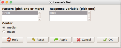
Figure 4. Screenshot menu options R Commander Levene’s test.
Select the median and the factor variable (in our case “Strain”) and the numeric outcome variable (“Bites”), then click OK button.
Tapply(bites ~ strain, var, na.action=na.omit, data=mice.aggression) # variances by group
inbred outbred
   0.8     7.2

leveneTest(bites ~ strain, data=mice.aggression, center="median")
Levene's Test for Homogeneity of Variance (center = median)
      Df F value  Pr(>F)
group  1       4 0.07339 .
      10
---
Signif. codes:  0 '***' 0.001 '**' 0.01 '*' 0.05 '.' 0.1 ' ' 1
End of R output
Compare the p-values. In both cases — F test and Levene’s test — we’re testing the same hypothesis (equal variances), but the p-values do not agree between the parametric F test and the nonparametric Levene’s test! If we were to go by the results of the F test, p-value was 0.031, less than out Type I error of 5% and we would tentatively conclude that the assumption of equal variances may not apply. On the other hand, if we go with the Levene’s test the p-value was 0.074, which is greater than our Type I error rate of 5% and we would therefore conclude the opposite, that the assumption of equal variances might apply! Both conclusions can’t hold, so which test result of equal variances do we prefer, the parametric F test or the nonparametric Levene’s test? Answer — we’d go with Levene’s because the F test is parametric and, therefore, also assumes normality.
Cahoy’s bootstrap method
Draft. Cahoy (2010). Variance-based statistic bootstrap test of heterogeneity of variances. we discuss bootstrap methods in Chapter 19.2; in brief, bootstrapping involves resampling the dataset and computing a statistic on each sample. This method may be more powerful, that is, more likely to correctly reject the null hypothesis when warranted, compared to Levene’s test.
for now, install package testequavar.
Function for testing two samples.
equa2vartest(inbred, outbred, 0.05, 999)
R output
[[1]]
[1] "Decision: Reject the Null"
$Alpha
[1] 0.05
$NumberOfBootSamples
[1] 999
$BootPvalue
[1] 0.006
The output “Decision: Reject the Null” reflects output from a box-type acceptance region.
Compare results from Levene’s test: p-value 0.07339 suggests accept hypothesis of equal variances, whereas bootstrap method indicates variances heterogenous, ie, reject equal variance hypothesis. However, re-running the test without setting the seed for R’s pseudorandom number generator will result in different p-values. For example, I re-ran Cahoy’s test five times with the following results:
0.008
0.006
0.002
0.01
0.004
Questions
- Test assumption of equal variances by Bartlett’s method and by Levene’s test on
OliveMomentvariable from the Comet tea data set introduced in Chapter 12.1. Do the methods agree? If not, which test result would you choose?- BONUS. Retest homogeneous variance hypothesis by
equa3vartest(Copper.Hazel, Copper, Hazel, 0.05, 999). Reject or fail to reject the null hypothesis by bootstrap method?
- BONUS. Retest homogeneous variance hypothesis by
- Test assumption of equal variances by Bartlett’s method and by Levene’s test on
Heightfrom the O’hia data set introduced in Chapter 12.7. Do the methods agree? If not, which result would you choose?- BONUS. Retest homogeneous variance hypothesis by
equa3vartest(M.1, M.2, M.3, 0.05, 999). Reject or fail to reject the null hypothesis by bootstrap method?
- BONUS. Retest homogeneous variance hypothesis by
Quiz Chapter 13.4
Tests for Equal Variances
R code reminders
The bootstrap method expects the variables in unstacked format. A simple method to extract the variables from the stacked data is to use a command like the following. For example, extract OliveMoment values for Copper-Hazel treatment.
Copper.Hazel <- cometTea$OliveMoment[1:10]
For Copper, Hazel, replace above with [11:20], and [21-30] respectively. Note: changed variable name from Copper-Hazel to Copper.Hazel. The hyphen is a reserved character in R.
Chapter 13 contents
10.2 – Digging deeper into t-test Plus the Welch test
Introduction
We need to spend some more time with the independent sample t-test; by tearing it apart, we can learn about how parametric tests work in general.
Our assumptions for the independent sample t-test are like the one-sample t-test the data must be continuous and normally distributed (one of our standard assumptions for parametric tests, see Chapter 13). The formula is very similar to the one-sample t-test, except that now we have two sample means and the formula for the standard error (SE) has also changed.

We see that the test statistic t is large if the numerator is large compared to the denominator. Large values of t will be evidence in favor of rejecting the null hypothesis.
The numerator is straightforward: we subtract one sample mean from the other — if there is no difference between the samples, then this difference will be close to zero.
The denominator requires additional discussion. What is it called? It is the pooled standard error of the mean (pooled SEM). Provided the assumption of equal variances holds — an additional standard assumptions for parametric tests, see Chapter 13 — then sample variances estimate the population variance and we can use this information to our advantage to best test the hypothesis about the sample means. In other words, we don’t have to lose a degree of freedom to account for differences in variability for the two groups (see Welch test). More degrees of freedom means more statistical power to test the null hypothesis and at the same time, more confidence that the test is performing to its best.
Lets break down the pooled standard error of the mean in order to see how the assumption of equal variances affects the t-test. We assume that 
Recall that

Now we want a “pooled SE” that is the pooled standard error for both samples. The variance of the difference between the means can be written as
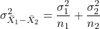
First we need to calculate the pooled variance. where v1 and v2 are degrees of freedom for sample one and sample two, respectively.
Note 1This is just simply a combined formula of the sample variance.
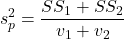
What is SS? The sum of squares , where SS1 and SS2 refer to sum of squares for each of the two groups.
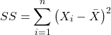
You should recognize SS from your definition of the sample variance, Chapter 3.3.
And the standard error for the difference between two means can now be written as So the 2-sample t-test can be written to reflect the pooled sample standard error of the difference between two sample means. We can see how unequal sample size is accommodated by the t-test.
Conducting the test by hand follows the same form as the one-sample t-test. Find the degrees of freedom (DF), but now for each sample.
Finally we evaluate with the critical value in Table (Appendix, Table of Student’s t distribution) and compare the t test statistic against the critical value with the appropriate degrees of freedom.
Because this is the t-test, again, we are assuming that the variances are the same between the two populations (homoscedasticity) and this allows us to pool the variance. As it turns out, the T-test is not overly sensitive to other deviations from the assumptions, but if the variances are in fact different, then the standard formula may yield incorrect Type I error rates compared to stated probability level (α).
However, it would be poor statistical choice to use a test where there are alternatives. This is why in part that R (Rcmdr) sets as the default for the t-test that variances are unequal! In fact, R does not do a t-test unless you change the default to assume equal variances, which, as we now know, is the t-test.
Welch test
What to do when assumptions to t-test are not met? Many options have been proposed, and Welch’s approximate t is a good alternative to the two-sample t-test — it would be appropriate if the normal assumption still held.
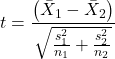
The degrees of freedom for the Welch’s test are now
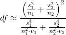
Note 2: The Welch test removes the pooled estimate of the standard error, replaces with both variance estimates directly.
As a default option, R and Rcmdr uses a variation of Welch’s test when you select to do the t-test without making the assumption of equal variance (Fig 1).
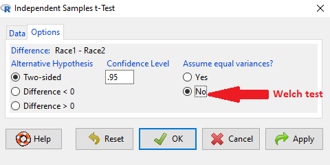
Figure 1. Screenshot Rcmdr t-test options. Default is “No” for Assume equal variances, ie, the Welch test.
The Welch test is not a nonparametric test, it is a different formulation of the t-test.
Justification for beginning with t-test
It’s unlikely that you will need the t-test in today’s research climate. Data sets are large, experiments are complex with multiple variables and samples. Why do we have to consider the t-test, and then a separate test in the case for unequal sample size? I view it as a teaching moment. It makes the general point that ALL statistical tests make assumptions about how the calculations are done and as to the nature of the data set.
This is our first experience with what to do if there is a violation of an assumption of parametric tests (see Chapter 13). Here, the assumption is that the two groups have equal sample size. When they do not, the standard t-test tends to biased estimates. On the other hand, if the assumptions are met, the standard test is the best test because it has more power to do what we intended — that is, it is best at the actual test of the null hypothesis! Take heart — this point is not always appreciated even by scientists (cf. Fagerland 2012).
Note 3: Expert advice will differ here, but you can always calculate the test statistic, even if the assumptions do not hold. The problem, the concern is with the interpretation.
Let’s us approach the problem of violation of assumptions in a couple of ways as an introduction to how, in general, to approach choice of statistical tests.
- Power of a test. Much current statistical research focuses on learning about how a particular statistical test works when assumptions are violated. Thus, in addition to learning what tests are designed to do, we need to consider the effects of violations of assumptions on the performance of the test (namely, is the Type I error at the stated alpha level?). This is a matter of statistical power; power of a test reflects how able the test is to get you the correct result even if assumptions are violated. Often tests perform well if sample sizes are large despite violation of assumptions. We mention without proving that the 2-sample T-test is robust to violations of normality assumption, to requirement for equal sample size, and even to unequal variances. But good experimental design attempts to meet the assumptions because the test does better!
- Alternate forms of some tests are available to handle some aspects of test violations. For example, the simple 2-sample T-test can be modified to accommodate different variances (Welch’s formula). Or you must find a different test (eg, nonparametric tests).
In conclusion, all tests begin with consideration of the assumptions. In some cases we can test our assumptions. For example, we learned about testing the assumption of normal distributions of sample data. We can also test the assumption of equal variances.
Questions
- Consider a clinical trial in which resting blood pressure is recorded on hypertensive subjects at the start of the trial, then 6 weeks after subjects have received daily supplements of flaxseed. Thus, for each subject there are two measures of blood pressure, BEFORE and AFTER.
- Write the null hypothesis
- Write the alternative hypothesis
- Justify why or why not the hypothesis should be two tailed. Explain why or why not an independent sample t-test may be used to compare groups.
Quiz Chapter 10.2
Digging deeper into t-test Plus the Welch test
Chapter 10 contents
- Introduction
- Compare two independent sample means
- Digging deeper into t-test Plus the Welch test
- Paired t-test
- References and suggested reading