20.15 — Meta-analysis
Introduction
Meta-analysis is a type of systematic review (Greenhalgh 1997, Akobeng 2005), a statistical method used to combine the results from multiple independent studies that addressed the same topic. By combining studies, the goal is to calculate a pooled estimate as a measure of overall effectiveness of the treatment. The underlying logic is that multiple studies draw subjects from the same reference population, thus, combining data provides a more powerful test of the hypothesis.
Meta-analysis can increase the overall sample size, which improves the study’s ability to detect an effect if one exists. So, how to combine results from different studies ostensibly addressing the same hypothesis? Inevitably, some subjectivity will come into decisions about including or excluding studies — the goal is to identify quality studies, which may have conflicting conclusions and test whether a single conclusion of effectiveness is warranted based on a summary of evidence.
Meta-analysis is now a routine type of study, conducted in multiple disciplines, including biomedical field (eg, Cochrane Reviews, more than 15K since 1993, Anderson et al 2024), and environmental studies (eg, Resende et al 2021), and sports science (eg, Miyamoto-Mikami et al 2018).
In general, meta-analysis studies return the combined effect size –the single, pooled effect across all included studies — of an intervention and the heterogeneity among the studies — how consistent measured differences. Models may be fixed effects — that is, any observed differences among studies are due to chance or sampling error — or random effects — the true effect size varies from study to study and that these effects are drawn from a distribution.
The purpose of this page is to provide a basic overview and an introduction to the meta-analysis approach. We previously introduced the Cochran’s Q test aka heterogeneity  test in Chapter 9.4. The chi-square test test asks whether results from combined studies are consistent. After discussing inclusion criteria, we provide plotting techniques and additional statistical tests for heterogeneity of studies.
In Chapter 12.4, we introduced a simple meta-analysis combining ten separate one sample t-tests of the hypothesis that inbred mice and genetically diverse mouse strains do not differ for average lifespan. P-values were combined and we used Fisher’s method to evaluate the hypothesis.
Note 1: The most robust and recommended method for meta-analysis is to use effect sizes (eg, standardized mean differences, odds ratios, risk ratios) and their corresponding standard errors or confidence intervals (Nakagawa and Cuthill 2007). This approach avoids the limitations of arbitrary p-value thresholds and provides a more complete picture of the effect’s magnitude and precision.
Selection criteria
Any project, whether an observational study or an experiment, starts with a question that is modified into one or more testable hypothesis. We don’t collect the data then speculate about causes for perceived patterns that may appear. Rather, pattern recognition process can be used to generate hypotheses subject to future testing. Our example was about lifespan and genetic background and genetic diversity: Longevity refers to the capacity to live a long life whereas lifespan is the maximum amount of time an individual can live. We ask if genetic diversity increases longevity across a population; specific genetic background is linked to an individual’s predisposition to long life.
Given the importance such work has in clinical research, as you can imagine, there is plenty of advice and suggested guidelines for how to proceed. Of note, review systematic review Population, Intervention, Comparison, Outcome (PICO) guidelines (Schardt et al 2007). Additionally, see the Cochrane Handbook (2024).
With a clear hypothesis in hand, for both systematic review and meta-analysis, the study begins with a search of the published literature. Search results from the query “inbred mice strain lifespan,” in Pubmed returned about 1134 publications; replacing “longevity” for “lifespan,” returned 654 publications. We want primary literature, not reviews, so we add NOT (Review[Publication Type]) to the query: 1080 and 617, respectively. Further restricting the pool by restricting range to last ten years returned a manageable 197 and 116 results, respectively. We can begin selecting our data from the studies. We now have to decide whether all or only some meet our standards for consideration. Of course, this is not the same thing as looking at the results and selecting only the studies that confirm our thinking! Ideally, reporting of both positive (large effect size, small p-value) and negative (small effect size, large p-value) studies can — and should — be included. Our goal, combine the results of multiple independent studies on the same topic to reach a more powerful and reliable conclusion than a single study could provide.
Note 2: Publication bias concerns likely overestimates of effect size for meta-analysis, just as the tendency for reporting only “statistically significant” p-values (Ioannidis 2008).
Inclusion criteria are the requirements a study must meet to be considered for the review; exclusion criteria are the specific reasons a study is disqualified. Decisions about which studies to include consider demographics, intervention type, and study design. For example, the review may focus only on RCT studies. Likely, the review is focused on experimental work and so, excluding previous systematic reviews would be an example of an exclusion criteria. At the same time we need to be transparent about our approach; that includes defining a clear research question, establishing strict inclusion/exclusion criteria, conducting a comprehensive literature search across multiple databases, and performing a rigorous data extraction and quality assessment of included studies (Meline 2006, Paldam 2015, Cochrane Handbook). For our lifespan and genetic diversity example I found two studies that met my criteria: the studies needed multiple inbred strains or outbred strains and the raw data needed to be available. Two studies met this need: Yuan et al (2009) and Mullis et al (2025).
An imperfect example. To practice applying selection and exclusion criteria for a meta-analysis, I ran a PubMed search using the keywords botox migraine. I limited the results to clinical trials published within the past five years, which gave me 14 papers. I read the abstracts and decided to include studies only if they had a control group, focused on patients with chronic migraine, and reported an exact p-value instead of just saying “P < 0.05.” Table 1 shows what I found, including the PubMed link for each paper, whether it was included, the sample size, the p-value, and my comments on why any studies were excluded.
Table 1. Example data collection for meta-analysis, topic botox and treatment of chronic migraines.
| paper | Include | N | p-value | Why exclude? |
|---|---|---|---|---|
| https://pubmed.ncbi.nlm.nih.gov/37499085/ | No | review | ||
| https://pubmed.ncbi.nlm.nih.gov/38982666/ | Yes | 1384 | 0.01 | |
| https://pubmed.ncbi.nlm.nih.gov/37994890/ | No | 209 | 0.155 | no control group |
| https://pubmed.ncbi.nlm.nih.gov/41091731/ | No | 775 | > 0.05 | no CI, no exact p-value |
| https://pubmed.ncbi.nlm.nih.gov/34404257/ | No | 32 | 0.03 | within subjects design, no control group |
| https://pubmed.ncbi.nlm.nih.gov/37315247/ | Yes | 209 | 0.365 | |
| https://pubmed.ncbi.nlm.nih.gov/33722518/ | No | 60 | < 0.001 | within subjects design, no control group, no exact p-value |
| https://pubmed.ncbi.nlm.nih.gov/36189948/ | No | 0.092 | no sample size, no control | |
| https://pubmed.ncbi.nlm.nih.gov/36189948/ | No | 0.174 | no sample size, no control | |
| https://pubmed.ncbi.nlm.nih.gov/35166150/ | No | method paper | ||
| https://pubmed.ncbi.nlm.nih.gov/33106278/ | Yes | 15 | 0.038 | |
| https://pubmed.ncbi.nlm.nih.gov/37235358/ | No | 139 | < 0.0001 | no CI, no exact p-value |
| https://pubmed.ncbi.nlm.nih.gov/35064733/ | No | overuse, not migraine | ||
| https://pubmed.ncbi.nlm.nih.gov/33241323/ | No | PTH, not migraine | ||
| https://pubmed.ncbi.nlm.nih.gov/32873093/ | No | no control group |
That leaves only three papers, not enough for a meta-analysis. By changing years from five to ten, 40 papers were available to search. By removing all time restrictions, 109 papers were returned since year 2000. Medical use of botox dates to the 1970s (Scott 2023).
R packages
metafor package: provides extensive functions for calculating various effect sizes, fitting different statistical models (e.g., fixed- and random-effects, mixed-effects), conducting meta-regression, and generating numerous meta-analytical plots.
See also metaforGUI package which provides a Graphical User Interface (GUI) for the R metafor Package.
meta package: provides user-friendly and comprehensive collection of functions for conducting standard meta-analyses.
Much has been written about how to conduct meta-analysis and caveat emptor — readers should be on notice that I present here just a fraction of the “how to” and pitfalls of meta-analysis. Interested readers should see Doing meta-analysis with R: A hands-on guide by M. Harrer et al (2021).
I2 or I-squared test
In a meta-analysis, the I-squared test  quantifies the percentage of total variation in a set of study results that is due to differences between studies rather than random sampling error (chance). An of 0% means all variation is due to chance, while a higher percentage indicates that differences between studies are a significant source of variation. As a reminder, the test returns a p-value that can be used to interpret whether that heterogeneity is statistically significant. We run our life span of inbred and genetically diverse outbred mouse strains example in Chapter 12.4; the p-value was small — we used Fisher’s method p-value combination approach to test the main hypothesis.
Here, we calculate ; we first need the effect size; Cohen’s d (Chapter 11.4) will do.
Table 1. Updated Table 1 from Chapter 12.4.
| Strain | n | mean | sd | cohen’s d | V(d) |
| 129S1/SvImJ | 32 | 787.4 | 159.16 | 0.045 | 0.191 |
| A/J | 32 | 630.7 | 130.20 | 1.26 | 0.04 |
| BALB/cByJ | 32 | 734.4 | 154.43 | 0.389 | 0.0368 |
| BUB/BnJ | 24 | 611.3 | 218.34 | 0.839 | 0.0485 |
| C3H/HeJ | 29 | 724.1 | 131.48 | 0.536 | 0.0403 |
| C57BL/6J | 29 | 855.7 | 185.34 | 0.330 | 0.0399 |
| CBA/J | 30 | 622.9 | 181.95 | 0.943 | 0.0405 |
| FVB/NJ | 26 | 750.3 | 230.11 | 0.192 | 0.0438 |
| P/J | 32 | 676.0 | 178.82 | 0.663 | 0.0374 |
| SWR/J | 31 | 831.9 | 181.31 | 0.206 | 0.0376 |
The effect size ranged from practically no difference (Cohen’s d of 4.5%) to substantial effect on average lifespan of inbred vs outbred strains (Cohen’s d of 126%). The simple average of the Cohen’s d values was 0.541; a weighted average accounting for differences in variance needs to be applied. Regardless, the statistic we want is the coefficient from meta-regression, which indicates how a change in that predictor relates to the effect size.
Note 3: The greatest effect size — difference in average lifespan — was reported for the A/J strain — this strain is primarily used in cancer research because of its susceptibility to cancers. The smallest effect size was for the 129S1/SvImJ strain, which is used for creating genetically modified mice.
With effect size calculated, we proceed to get . We use rma() from metafor package. This function performs several tests: a fixed-effects model and therefore we test a model where we assume all studies found the exact same effect, a random-effects model where the assumption is that effects are similar but vary across studies, plus a mixed-effects model uses a combination of both, and finally, a meta-regression. The meta-regression uses the data from those studies to try and explain why the results differ.
R code
library(metafor)
strains <- 1:10
my_effsize <- c(0.0446092, 1.258065, 0.3891731, 0.8390583,
0.5354427, 0.3302039, 0.9431162, 0.192082, 0.6626776, 0.2062765)
my_sample <- c(32, 32, 32, 24, 29, 29, 30, 26, 32, 31)
my_varC <- (my_effsize^2)/(2*my_sample)
myData <- data.frame(strains, my_effsize, my_sample, my_varC)
rma(yi = my_effsize, vi = my_varC, data = myData)
R output
Random-Effects Model (k = 10; tau^2 estimator: REML)

tau^2 (estimated amount of total heterogeneity): 0.1299 (SE = 0.0643)
tau (square root of estimated tau^2 value): 0.3604
I^2 (total heterogeneity / total variability): 99.15%
H^2 (total variability / sampling variability): 117.11

Test for Heterogeneity:
Q(df = 9) = 390.9415, p-val < .0001

Model Results:

estimate     se   zval   pval  ci.lb  ci.ub
  0.5208 0.1169 4.4558 <.0001 0.2917 0.7499 ***
---
Signif. codes: 0 ‘***’ 0.001 ‘**’ 0.01 ‘*’ 0.05 ‘.’ 0.1 ‘ ’ 1
Interpretation.
With an of 99%, which suggests a very high degree of heterogeneity among the comparison between the DO strain and the ten inbred strains for life span. As before, the heterogeneity or Q test was highly statistically significant, suggests that the observed variability is larger than what would be expected due to chance alone. Thus, all of the variability in the observed effects comes from between-strain differences, not random chance — it also justifies use of a random effects model, not a fixed model. Strain A/J, with the greatest difference in lifespan compared to the DO strain, is recognized for its susceptibility to carcinogenic tumors
From the meta regression, the coefficient was 0.52 — inbred strain membership was associated with change in the size of the effect. We conclude that in general, the genetically inbred strains differ substantially for average lifespan compared to the genetically variable DO strain: The true average effect was somewhere between 0.2917 and 0.7499.
Our results conform to our expectations — longevity is likely affected by a combination of effects from many genes along with an individual’s genetic background and interaction with the environment, cf discussion in Mullis et al (2025).
Forest plot of effect size.
A forest plot visually summarizes results from multiple studies, showing each study’s effect size (eg, odds ratio, mean difference, Cohen’s d) and variance or confidence interval as squares and lines, plus the overall pooled estimate (diamond). It helps quickly assess study consistency (heterogeneity), see individual study contributions, and determine if the combined evidence points to a significant overall effect.
For example, our inbred strains vs the outbred DO strain for lifespan shows a clear, overall effect (Fig 1). The diverse genetic strain lifespan is significantly greater than the majority of inbred strains, and the combined effect is about 0.5.
R code
library(metafor)
myData <- data.frame(
Strains = paste("Strains", c("129S1/SvImJ", "A/J", "BALB/cByJ", "BUB/BnJ",
"C3H/HeJ", "C57BL/6J", "CBA/J", "FVB/NJ", "P/J", "SWR/J")),
cohenD = c(0.045, 1.26, 0.389, 0.839, 0.536, 0.33, 0.943, 0.192, 0.663, 0.206),
cohenV = c(0.1910, 0.0400, 0.0368, 0.0485, 0.0403, 0.0399, 0.0405, 0.0438, 0.0374, 0.0376)
)

res2 <- rma(cohenD, cohenV, data = myData, method="REML")
# str(res2)

forest(res2,
slab = myData$Strains,
xlab = "Cohen's d")
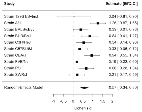
Figure 1. Forest plot, Cohen’s effect size lifespan differences among inbred strains of mice compared to outbred strain.
Questions
1. What’s the difference between a literature review and a systematic review?
2. For which kinds of research goals would a meta-analysis be more appropriate than a systematic review?
Quiz Chapter 20.15
Meta-analysis
References and suggested readings
Akobeng, A. K. (2005). Understanding systematic reviews and meta-analysis. Arch Dis Child, 90:845-848.
Andersen, M. Z., Zeinert, P., Rosenberg, J., & Fonnes, S. (2024). Comparative analysis of Cochrane and non-Cochrane reviews over three decades. Systematic Reviews, 13, 120.
Cochrane reviews, Cochrane Library. (2025). https://www.cochranelibrary.com/
Greenhalgh, T. (1997). How to read a paper: Papers that summarise other papers (systematic reviews and meta-analyses). BMJ, 315(7109), 672–675.
Gurevitch, J., Koricheva, J., Nakagawa, S., & Stewart, G. (2018). Meta-analysis and the science of research synthesis. Nature, 555(7695), 175–182.
Hansen, C., Steinmetz, H., & Block, J. (2022). How to conduct a meta-analysis in eight steps: A practical guide. Management Review Quarterly, 72(1), 1–19.
Harrer, M., Cuijpers, P., Furukawa, T.A., & Ebert, D.D. (2021). Doing Meta-Analysis with R: A Hands-On Guide. Boca Raton, FL and London: Chapman & Hall/CRC Press. Link to website.
Ioannidis, J. P. A. (2008). Why Most Discovered True Associations Are Inflated. Epidemiology, 19(5), 640.
Higgins JPT, Thomas J, Chandler J, Cumpston M, Li T, Page MJ, Welch VA (editors). Cochrane Handbook for Systematic Reviews of Interventions version 6.5 (updated August 2024). Cochrane, 2024. Available from www.cochrane.org/handbook.
Meline, T. (2006). Selecting studies for systemic review: Inclusion and exclusion criteria. Contemporary Issues in Communication Science and Disorders, 33(Spring), 21–27.
Miyamoto-Mikami, E., Zempo, H., Fuku, N., Kikuchi, N., Miyachi, M., & Murakami, H. (2018). Heritability estimates of endurance-related phenotypes: A systematic review and meta-analysis. Scandinavian Journal of Medicine & Science in Sports, 28(3), 834–845.
Mullis, M. N., Wright, K. M., Raj, A., Gatti, D. M., Reifsnyder, P. C., Flurkey, K., Archer, J. R., Robinson, L., Di Francesco, A., Svenson, K. L., Korstanje, R., Harrison, D. E., Ruby, J. G., & Churchill, G. A. (2025). Analysis of lifespan across diversity outbred mouse studies identifies multiple longevity-associated loci. Genetics, 230(4), iyaf081.
Nakagawa, S., & Cuthill, I. C. (2007). Effect size, confidence interval and statistical significance: A practical guide for biologists. Biological Reviews, 82(4), 591–605.
Paldam, M. (2015). Meta-analysis in a nutshell: Techniques and general findings. Economics, 9(1), 20150011.
Resende, P. S., Viana-Junior, A. B., Young, R. J., & Azevedo, C. S. (2021). What is better for animal conservation translocation programmes: Soft- or hard-release? A phylogenetic meta-analytical approach. Journal of Applied Ecology, 58(6), 1122–1132.
Schardt, C., Adams, M. B., Owens, T., Keitz, S., & Fontelo, P. (2007). Utilization of the PICO framework to improve searching PubMed for clinical questions. BMC Medical Informatics and Decision Making, 7, 16.
Scott, A. B., Honeychurch, D., & Brin, M. F. (2023). Early development history of Botox (onabotulinumtoxinA). Medicine, 102(Suppl), e32371.
van Aert, R. C. M., Wicherts, J. M., & van Assen, M. A. L. M. (2016). Conducting Meta-Analyses Based on p Values. Perspectives on Psychological Science, 11(5), 713–729.
Yuan, R., Tsaih, S.-W., Petkova, S. B., de Evsikova, C. M., Xing, S., Marion, M. A., Bogue, M. A., Mills, K. D., Peters, L. L., Bult, C. J., Rosen, C. J., Sundberg, J. P., Harrison, D. E., Churchill, G. A., & Paigen, B. (2009). Aging in inbred strains of mice: Study design and interim report on median lifespans and circulating IGF1 levels. Aging Cell, 8(3), 277–287.
Chapter 20 contents
- Additional topics
- Area under the curve
- Peak detection
- Baseline correction
- Surveys
- Time series
- Dimensional analysis
- Estimating population size
- Diversity indexes
- Survival analysis
- Growth equations and dose response calculations
- Plot a Newick tree
- Phylogenetically independent contrasts
- How to get the distances from a distance tree
- Binary classification
- Meta-analysis
9.4 – Heterogeneity chi-square tests
Planned comparisons and meta-analysis.
After finding evidence to reject the statistical null hypothesis, it may be appropriate to proceed to test a number of data sets against the same theoretical distribution. Provided these are planned comparisons, part of the experiment and not an exercise in data dredging (Norman 2014), you may proceed to test a series of nested models where groups are combined to make new groups for comparison. This approach is analogous to the post-hoc tests one may conduct after a statistically significant ANOVA (see Chapter 12.4) or when identifying a best-fit regression model (see Chapter 18.4).
Combining groups to make new comparisons — this scenario is consistent with a meta-analysis. A type of systematic review (Greenhalgh 1997, Akobeng 2005), meta-analysis is a statistical method that combines the results from multiple independent studies on the same topic to provide a more precise and robust overall conclusion. By combining studies, the goal is to calculate a pooled estimate as a measure of overall effectiveness of the treatment. Meta-analysis can increase the overall sample size, which improves the study’s ability to detect an effect if one exists. So, how to combine results from different studies ostensibly addressing the same hypothesis? Inevitably, some subjectivity will come into decisions about including or excluding studies — the goal is to identify quality studies, which may have conflicting conclusions and test whether a single conclusion of effectiveness is warranted based on a summary of evidence.
Here we introduce the Cochran’s Q test (Cochran 1954, Hoaglin 2016), aka a special case of the more general heterogeneity chi-square test. The null hypothesis is no significant difference in the proportion of “successes” across all groups being compared — any observed differences between the groups are just due to chance. The test statistic, Q, has a chi-square distribution with  degrees of freedom. A large Q value and small p-value suggest significant heterogeneity of results among the studies.
Note 1. As a reminder, “success” as an outcome category in epidemiology studies can represent any result depending on the study’s objective: survival, recovery, symptom improvement, or prevention of infection. The alternative outcome is generally referred to as “failure” (eg, death, non-recovery, no improvement, infection).
Heterogeneity tests ask whether results from combined studies are consistent; other tests exist, and are detailed in our special chapter on conducting meta-analysis. For example, I2 or I-squared test provides a measure of how much variation in the combined studies is due to true differences rather than by chance. In short, the I2 test quantifies how much — the percentage — the different studies agree, while the chi-square test returns a p-value that can be used to interpret whether that heterogeneity is statistically significant. We outline the basics of meta-analysis in Chapter 20.15. Other tests include DerSimonian-Laird test and Mandel-Paule test — these use the Q statistic and its distribution to estimate the between-study variance and provide better estimators with small sample size. Between-study variance is used to determine if a fixed-effect or a random-effects model (Chapter 12.3 and Chapter 14.3), is appropriate for the analysis. A random-effects model is used when significant heterogeneity is present (Higgins et al 2009).
Example.
Imagine a scenario where a population geneticist has collected allele (gene) frequency and genotype frequency data on single nucleotide polymorphisms (SNP) for the BRCA1 locus for three USA groups, African Americans, Asian Americans, and European Americans. Data of this kind can be obtained from the SNP database at NCBI (data retrieved 14 & 15 July 2014), and I collated several SNP involving a Cytosine base for Thymine base change (Table 1). The BRCA1 locus is on chromosome 17 and some of the hundreds of mutations found for this gene are associated with high risk of breast and or ovarian cancer (Couch and Weber 1996, Tram et al 2013).
Table 1. SNP of BRCA1 locus
| SNP | Population | n | C/C | C/T | T/T | C | T |
| rs1060915 | African American | 46 | 0.043 | 0.174 | 0,783 | 0.130 | 0.870 |
| Asian American | 48 | 0.083 | 0.625 | 0.375 | 0.396 | 0.604 | |
| European American | 48 | 0.167 | 0.458 | 0.375 | 0.396 | 0.604 | |
| rs3737559 | African American | 40 | 0.043 | 0.174 | 0.783 | 0.130 | 0.870 |
| Asian American | 48 | 0.083 | 0.625 | 0.292 | 0.396 | 0.604 | |
| European American | 48 | 0.167 | 0.458 | 0.375 | 0.396 | 0.604 | |
| rs799917 | African American | 124 | 0.048 | 0.258 | 0.694 | 0.177 | 0.823 |
| Asian American | 90 | 0.467 | 0.444 | 0.089 | 0.689 | 0.311 | |
| European American | 118 | 0.407 | 0.458 | 0.136 | 0.636 | 0.364 |
We may wish to test the combined data set to see if the large data set differs from Hardy Weinberg expectations before proceeding with a series of sample populations. By combining the data sets, we will be able to test whether one genotype is different from exception.
The goal then is to pool the data so that you have a more powerful test of the null hypothesis (remember our general discussion of statistical power and how increasing sample size increases your chances of correctly rejecting the null hypothesis).
For example, in our test of Hardy-Weinberg expectations (Example C), we calculated a  test of 7.8955. This test has k – 1 = 3 – 1 = 2 degrees of freedom. At alpha 5%, the critical value was 5.991 We clearly would reject the null hypothesis. But do we reject because of a difference in the aa, ab, or bb genotypes? Simply combine categories. Let’s test the homozygotes (aa and bb) versus the heterozygotes (ab).
Table 2. Worksheet
|
Categories
|
|||
| aa + bb | ab | n | |
|
Observed
|
66 | 34 | 100 |
|
Expected
|
52 | 48 | 100 |
 |
 |
||
With one degree of freedom, we clearly reject the null hypothesis because the critical value at 5% and one degree of freedom is equal to 3.841. To get the p-value, use
pchisq(7.852,df=1,lower.tail=FALSE)
which will return
[1] 0.005076452
Oh, and what was the null hypothesis? That there was an equal number of homozygotes and heterozygotes.
Other tests would be possible here, but the point is that you can dissect an experiment to determine which group is causing you to reject the null original hypothesis. While this is an important tool, you should also consider issues of apriori and aposterori decisions in experiments.
Questions.
1. The SNP rs1799971 (A > G) in the μ-opioid receptor (MOR) is associated with opioid dependency. Allele frequencies for different populations are provided in the table. Global frequency for A at this SNP is 0.188 (therefore frequency of G is 0.812).
| Population | n | A | G |
|---|---|---|---|
| African American | 32510 | 0.97 | 0.03 |
| Central American | 2450 | 0.81 | 0.19 |
| European | 18872 | 0.86 | 0.14 |
| Native American | 1260 | 0.86 | 0.14 |
| Native Hawaiian | 4534 | 0.75 | 0.25 |
| South Asian | 856 | 0.59 | 0.41 |
- Combine the data sets and test whether genotype frequency is different from the reported global exception.
- Test each population separately.
2. A behavioral ecologist studies the effect of three diets (high-protein, high-carbohydrate, and mixed) on the growth rate of juvenile frogs. Before collecting any data, she writes a protocol stating that she will compare only the high-protein vs mixed diet, based on a specific hypothesis about amino acid availability.
After analyzing the data, she also notices that frogs on the high-carbohydrate diet seem smaller, so she performs several additional pairwise comparisons that were not part of her original plan, reporting only the ones that are statistically significant.
Which statement best distinguishes the planned comparison from data dredging (p-hacking)?
A. The planned comparison is valid because it uses a larger sample size, while data dredging uses small samples.
B. The planned comparison was specified ahead of time based on a biological hypothesis, while data dredging involves unplanned tests added after seeing the data to search for significant results.
C. The planned comparison uses ANOVA, while data dredging uses regression.
D. The planned comparison must always produce a significant result, while data dredging never does.
Quiz Chapter 9.4
Heterogeneity chi-square tests