9.3 – Yates continuity correction
Introduction
Yates continuity correction: Most statistical textbooks at this point will note that critical values in their table (or any chi-square table for that matter) are approximate, but don’t say why. We’ll make the same directive — you may need to make a correction to the  for low sample numbers. It’s not a secret, so here’s why.
We need to address a quirk of the test: the chi-square distribution is a continuous function (if you plotted it, all possible values between, say, 4 and 3 are possible). But the calculated statistics we get are discrete. In our HIV-HG co-infection problem from the previous subchapter, we got what appears to be an exact answer for P, but it is actually an approximation.
We’re really not evaluating our test statistic at the alpha levels we set out. This limitation of the goodness of fit statistic can be of some consequence — increases our chance to commit a Type I error — unless we make a slight correction for this discontinuity. The good news is that the does just fine for most df, but we do get concerned with it’s performance at df = 1 and for small samples.
Therefore, the advice is to use a correction if your calculated is close to the critical value for rejection/acceptance of the null hypothesis and you have only one df. Use the Yate’s continuity correction to standard calculation,  .
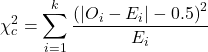
For the 2×2 table (Table 1), we can rewrite Yates correction

Our concern is this: without the correction, Pearson’s test statistic will be biased (eg, the test statistic will be larger than it “really” is), so we’ll end up rejecting the null hypothesis when we shouldn’t (that’s a Type I error). This becomes an issue for us when p-value is close to 5%, the nominal rejection level: what if p-value is 0.051? Or 0.049? How confident are we in concluding accept or reject null hypothesis, respectively?
I gave you three examples of goodness of fit and one contingency table example. You should be able to tell me which of these analyses it would be appropriate to apply to correction.
More about continuity corrections
Yates suggested his correction to Pearson’s back in 1934. Unsurprisingly, new approaches have been suggested (eg, discussion in Agresti 2001). For example, Nicola Serra (Serra 2018; Serra et al 2019) introduced
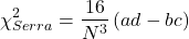
Serra reported favorable performance when sample size was small and the expected value in any cell was 5 or less.
R code
When you submit a 2X2 table with one or more cells less than five, you could elect to use a Fisher exact test, briefly introduced here (see section 9.5 for additional development), or, you may apply the Yates correction. Here’s some code to make this work in R.
Let’s say the problem looks like Table 1.
Table 1. Example 2X2 table with one cell with low frequency.
| Yes | No | |
| A | 8 | 12 |
| B | 3 | 22 |
At the R prompt type the following
library(abind, pos=15)
#abind allows you to combine matrices into single arrays
.Table <- matrix(c(8,12,3,22), 2, 2, byrow=TRUE)
rownames(.Table) <- c('A', 'B')
colnames(.Table) <- c('Yes', 'No') # when you submit, R replies with the following table
.Table  # Counts
 Yes No
A  8 12
B  3 22
Here’s the command; the default is no Yates correction (ie, correct=FALSE); to apply the Yates correction, set correct=TRUE.
.Test <- chisq.test(.Table, correct=TRUE)
Output from R follows
.Test
    Pearson's Chi-squared test with Yates' continuity correction
data:  .Table
X-squared = 3.3224, df = 1, p-value = 0.06834
Compare without the Yates correction
.Test <- chisq.test(.Table, correct=FALSE)
.Test
    Pearson's Chi-squared test
data:  .Table
X-squared = 4.7166, df = 1, p-value = 0.02987
Note that we would reach different conclusions! If we ignored the potential bias of the un-corrected we would be tempted to reject the null hypothesis, when in fact, the better answer is not to reject because Yates-corrected p-value is greater than 5%.
Just to complete the work, what does the Fisher Exact test results look like (see section 9.5)?
fisher.test(.Table)
    Fisher's Exact Test for Count Data
data:  .Table
p-value = 0.04086
alternative hypothesis: true odds ratio is not equal to 1
95 percent confidence interval:
0.9130455 32.8057866
sample estimates:
odds ratio
  4.708908
Which to use? The Fisher exact test is just that, an exact test of the hypothesis. All possible outcomes are evaluated and we interpret the results as likely as p=0.04086 if there is actually no association between the treatment (A vs B) and the outcome (Yes/No) (see section 9.5).
Questions
- With respect to interpreting results from a test for small samples, why use the Yates continuity correction?
- Try your hand at the following four contingency tables (a – d). Calculate the test, with and without the Yates correction. Make note of the p-value from each and note any trends.
(a)
| Yes | No | |
| A | 18 | 6 |
| B | 3 | 8 |
(b)
| Yes | No | |
| A | 10 | 12 |
| B | 3 | 14 |
(c)
| Yes | No | |
| A | 5 | 12 |
| B | 12 | 18 |
(d)
| Yes | No | |
| A | 8 | 12 |
| B | 3 | 3 |
3. Ch09.1, Question 1 provided an example of a count from a small bag of M&Ms. Apply the Yates correction to obtain a better estimate of p-value for the problem. The data were four blue, two brown, one green, three orange, four red, and two yellow candies.
- Construct a table and compare p-values obtained with and without the Yates correction. Note any trend in p-value
Quiz Chapter 9.3
Yates continuity correction
Chapter 9 contents
7.5 – Odds ratio
What are the odds.
We introduced the concept of odds 7.1 — Epidemiology definitions. As a reminder, odds are a way to communicate the chance (likelihood) that a particular event will take place. Odds are calculated as the number of individuals with the event divided by the number of individuals without the event.
Odds ratio definition: is a measure of effect size for the association between two binary (yes/no) variables. It is the ratio of the odds of an event occurring in one group to the odds of the same event happening in another group. The odds ratio (OR) is a way to quantify the strength of association between one condition and another.
Note 1: Effect size — the size of the difference between groups — is discussed further in Chapter 9.2 and Chapter 11.4.
And note, it’s association, not correlation. In statistics, correlation is a specific kind of relationship (linear) among the variables, whereas “association” means there is some relationship between the variables without specifying the shape of the relationship.
How are odds ratios calculated? The probabilities are conditional; recall that conditional probability of some event A, given the occurrence of some other event B.
Let  equal probability of the event occurring (y = Yes) in A,
 equal probability of the event not occurring (n = No) in A,
 equal probability of the event occurring in B, and
 equal probability of the event not occurring in B.
| A | |||
| Yes | No | ||
| B | Yes | |
|
| No | |
|
|
These sum to one: 
The conditional probabilities are
| A | |||
| Yes | No | ||
| B | Yes |  |
 |
| No |  |
 |
|
and finally then, the odds ratio (OR) is
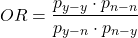
If you have the raw numbers you can calculate the odds ratio directly, too.
| A | |||
| Yes | No | ||
| B | Yes | a | b |
| No | c | d | |
and the odds ratio is then

or, equivalently

Example.
Comparing proportions is a frequent need in court. Gray (2002) provided an example from Title IX of the Education Act of 1972 case Cohen v. Brown University. Under the Act, discrimination based on gender is prohibited. The case concerned participation in collegiate athletics by women. The case data were that of the 5722 undergraduate students, 51% were women, but of the 987 athletes, only 38% were women. A mosaic plot shows graphically these proportions (Fig 1, males in red bars, females in yellow bars).
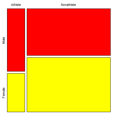
Figure 1. Mosaic plot of athletes to non-athletes in college. Males red, females yellow, data from Gray 2002.
Alternatively, use a Venn diagram to describe the distribution (Fig 2). Circles that overlap show regions of commonality.
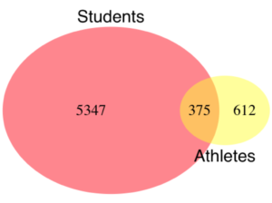
Figure 2. Venn Diagram of athletes to non-athletes in college. Female athletes (n = 375), male athletes (n = 612), data from Gray 2002.
where the orange region

R code for the Venn diagram was
library(VennDiagram)
area1 = 5722
area2 = 987
cross.area = 375
draw.pairwise.venn(area1,area2,cross.area,category=c("Students","Athletes"),
euler.d = TRUE, scaled = TRUE, inverted = FALSE, print.mode = "percent",
fill=c("Red","Yellow"),cex = 1.5, lty="blank", cat.fontfamily = rep("sans", 2),
cat.cex = 1.7, cat.pos = c(0, 180), ext.pos=0)
The question raised before the court was whether these proportions meet the demand of “substantially proportionate.” What exactly the law means by “substantially proportionate” was left to the courts and the lawyers to work out (Gray 2002). Title IX suggests that “substantially proportionate” is a statistical problem and the two sides of the argument must address the question from that perspective.
What is the chance that an undergraduate student was an athlete and female? 38% And the chance that an undergraduate student was an athlete and male? 62% Clearly 38% is not 62%; did the plaintiffs have a case?
Graphs like Figure 1 and Figure 2 help communicate but can’t provide a sense of whether the differences are important. Let’s start by looking at the numbers. Working with the proportions we have the following break down for numbers of students (Table 1) or as proportions (Table 2).
Table 1. Gray’s raw data displayed in a 2 x 2 format.
| Athletes | |||
| Yes | No | ||
| Undergraduates | Male | 612 | 2192 |
| Female | 375 | 2543 | |
Together, the numbers total 5,722.
The Odds Ratio (OR) would be

Or from the proportions (Table 2)
Table 2. Data from Table 1 as proportions.
| Athletes | |||
| Yes | No | ||
| Undergraduates | Male | 0.107 | 0.383 |
| Female | 0.066 | 0.444 | |
adding all of these frequencies together equal 1. Carry out the calculation of odds (Table 3), the conditional probabilities (in bold).
Table 3. Odds calculated from Table 2 inputs.
| Athletes | |||
| Yes | No | ||
| Undergraduates | Male | 0.218
|
0.782
|
| Female | 0.129
|
0.871
|
|
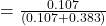
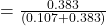
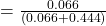
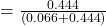
Calculate the odds ratio

Thankfully, whether we use the raw number format or the proportion format, we got the same results!
Odds ratio interpretation.
Because the Odds Ratio (OR) was greater than 1, males students were more likely to be athletes than female students. If there was no difference in proportion of male and female athletes, the odds ratio would be close to one. That is a test of statistical inference (eg, a contingency table), but for now, if one is included in the confidence interval, then this would be evidence that there was no difference between the proportions.
And in R? Simple enough, just create a matrix then apply the Fisher test. which we will discuss further in Chapter 9.5.
title9 <- matrix(c(612, 2192, 375, 2543), nrow=2))
fisher.test(title9)
and results
p-value < 2.2e-16
alternative hypothesis: true odds ratio is not equal to 1
95 percent confidence interval:
1.641245 2.185576
sample estimates:
odds ratio
1.893143
Thankfully, they agree. But note, we now have confidence intervals and a p-value, which we use to conduct inference: were the odds “significantly different from 1?” We would conclude, yes! Between the lower limit (1.64) and the upper limit (2.19), the value “1” was excluded. Moreover, the p-value at 2.2e-16 was much less than the standard type I error cut-off of 5% (see Chapter 8).
Before we leave the interpretation, sometimes a calculated odds-ratio is less than one. If our calculated odds ratio for the Title IX case described in Table 1 was less than 1, (say, the numbers were flipped, Table 4) we then the interpretation would be females were more likely to be athletes on college campus.
Table 4. Table 1 data, but order of entry changed.
| Athletes | |||
| Yes | No | ||
| Undergraduates | Female | 375 | 2543 |
| Male | 612 | 2192 | |
Now, calculating the odds via Fisher exact test, the odds ratio is less than one (0.53):
Fisher's Exact Test for Count Data
p-value < 2.2e-16
alternative hypothesis: true odds ratio is not equal to 1
95 percent confidence interval:
0.4575452 0.6092936
sample estimates:
odds ratio
0.5282222
Note this result is for the same data (Table 1 vs Table 4), just the order by which the groups are specified changed. Of course they are related to each other mathematically, and in a simple way. Note that taking the inverse (reciprocal) odds ratio.

will return the comparison we wanted in the first place — the odds a student athlete was male. As long as you keep track of the comparison, of the groups, it may be easier to communicate results when the reported odds ratio is greater than one.
Relative risk v. odds ratio.
We introduced another way to quantify this association as the Relative Risk (RR) and Absolute Risk Reductions in the previous section. Both can be used to describe the risk of the treatment (exposed) group relative to the control (nonexposed) group. RR is the ratio the treated to control group. OR is the ratio between odds of treated (exposed) and control (nonexposed). What’s the difference? OR is more general — it can be used in situations in which the researcher chooses the number of affected individuals in the groups and, therefore, the base rate or prevalence of the condition in the population is not known or is not representative of the population, whereas RR is appropriate when prevalence is known (this is a general point, but see Schechtman 2002 for a nice discussion).
The odds ratio is related to relative risk, but not over the entire range of possible risk. Odds of an event is simply the number of individuals with the event divided by the number without the event. Odds of an event therefore can range from zero (event cannot occur) to infinity (event must occur). For example, odds of eight (1.89:1) means that nearly two male students were student athletes at Brown University for every one female student.
In contrast, the risk of an event occurring is the number of individuals with the event divided by the total number of people at risk of having that event. Risk is expressed as a percentage (Davies et al 1998). Thus, for our example, odds of 1.89:1 correspond to a risk of 1.89 divided by (1 + 1.89) equals 65%.
To get the relative risk we can use

or 1.7% for our example.
In this example we could use either odds or relative risk; the key distinction is that we knew how many events happened in both groups. If this information is missing for one group (eg, control group of the case-control design), then only the odds ratio would be appropriate.
From cumulative wisdom in the literature (eg, Tamhane et al 2107), if prevalence is less than ten percent, OR ≈ RR. We can relate RR and OR as
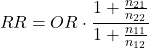
where n11 and n21 are the frequency with the condition for group 1 and group 2, respectively, and n12 and n22 are the frequency without the condition for group 1 and group 2, respectively. For the examples on this page group 1 is the treatment group and group 2 is the control group.
Hazard ratio
The hazard ratio is the ratio of hazard rates. Hazard rates are like the relative risk rates, but are specific to a period of time. Hazard rates come from a technique called Survival Analysis (introduced in Chapter 20.9). Survival analysis can be thought of as following a group of subjects over time until something (the event) happens. By following two groups, perhaps one group exposed to a suspected carcinogen vs. another group matched in other respects except the exposure, at the end of the trial, we’ll have two hazard rates: the rate for the exposed group and the rate for the control group. If there is no difference, then the hazard ratio will be one.
Hazard ratios are more appropriate for clinical trials; relative risk is more appropriate for observational studies.
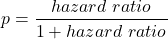
For a hazard ratio, it is often easier to think of it as a probability (between 0 to 1). To translate a hazard ratio to a probability use the following equation
Questions
- Distinguish between odds ratio, relative risk, and hazard ratio.
- Refer to problem 1 introduced in 7.4 – Epidemiology: Relative risk and absolute risk, explained.
Quiz Chapter 7.5
Odds ratio