8.2 – The controversy over proper hypothesis testing
Introduction
Over the next several chapters we will introduce and develop an approach to statistical inference, which has been given the title “Null Hypothesis Significance Testing” or NHST.
In outline, NHST proceeds with
- statements of two hypotheses, a null hypothesis, HO, and an alternative hypothesis, HA
- calculate a test statistic comparison of the null hypothesis (assuming some characteristic of data).
- The value of the test statistic is to be compared to a critical value for the test, identified for the assumed probability distribution at associated degrees of freedom for the statistical function, and assigned Type I error rate.
We will expand on these statements later in this chapter, so stay with me here. Basically, the null hypothesis is often a statement like the responses of subjects from the treatment and control groups are the same, eg, no treatment effect. Note that the alternative hypothesis, eg, hypertensive patients receiving hydalazine for six weeks have lower systolic blood pressure than patients receiving a placebo (Campbell et al 2011), would be the scientific hypothesis we are most interested in. But in the Frequentist NHST approach we test the null hypothesis, not the alternative hypothesis. This framework over proper hypothesis testing is the basis of the Bayesian vs Frequentist controversy.
Consider the independent sample t-test (see Chapter 8.5 and 8.6), our first example of a parametric test.

After plugging in the sample means and the standard error for the difference between the means, we calculate t, the test statistic of the t-test. The critical value is treated as a cut-off value in the NHST approach. We have to set our Type I error rate before we start the experiment, and we have available the degrees of freedom for the test, which follows from the sample size. With these in hand, the critical value is found by looking in the t-table of probabilities (or better, use R).
For example, what is the critical value of t-test with 10 degrees of freedom and Type I error of 5%?
In Rcmdr, choose Distributions → Continuous distributions → t distribution → t quantiles… (Fig 1).
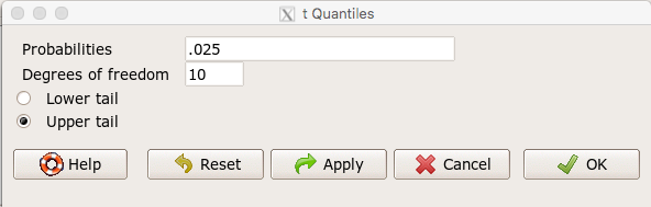
Figure 1. Screenshot t-quantiles Rcmdr menu.
Note we want Type I equal to 5%. Since there are two tails for our test, we divide 5% by two and enter 0.025 and select the Upper tail.
R output
> qt(c(.025), df=10, lower.tail=FALSE)
[1] 2.228139
which is the same thing we would get if we look up on the t-distribution table (Fig 2).
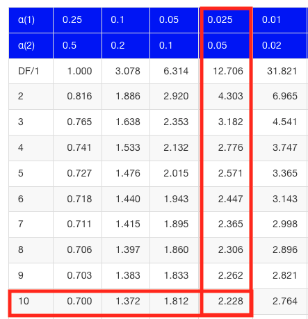
Figure 2. Screenshot of portion of t-table with highlighted (red) critical value for 10 degrees of freedom.
If the test statistic is greater than the critical value, then the conclusion is that the null hypothesis is to be provisionally rejected. We would like to conclude that the alternative hypothesis should favored as best description of the results. However, we cannot — the p-value simply tells us how likely our results would be obtained and if the null hypothesis was true. Confusingly, however, you cannot interpret the p-value as telling you the probability (how likely) that the null hypothesis is true. If however the test statistic is less than the critical value, then the conclusion is that the null hypothesis is to be provisionally accepted.
The test statistic can be assigned a probability or p-value. This p-value is judged to be large or small relative to an a priori error probability level cut off called the Type I error rate. Thus, NHST as presented in this way may be thought of as a decision path — if the test statistic is greater than the critical value, which will necessarily mean that the p value is less than the Type I error rate, then we make one type of conclusion (reject HO). In contrast, if the test statistic is less than the critical value, which will mean that the p-value associated with the test statistic will be greater than the Type I error rate, then we conclude something else about the null hypothesis. The various terms used in this description of NHST were defined in Chapter 8.3.
Sounds confusing, but, you say, OK, what exactly is the controversy? The controversy has to do whether the probability or p-value can be interpreted as evidence for a hypothesis. In one sense, the smaller the p-value, the stronger the case to reject the null hypothesis, right? However, just because the p-value is small — the event is rare — how much evidence do we have that the null hypothesis is true? Not necessarily, and so we can only conclude that the p-value is one part of what we may need for evidence for or against a hypothesis (hint: part of the solution is to consider effect size — introduced in Chapter 9.2 — and the statistical power of the test, see Ch 11). What follows was covered by Goodman (1988) and others. Here’s the problem. Consider tossing a fair coin ten times, with the resulting trial yielding nine out of ten heads (eg, a value of one, with tails equal to zero).
R code
set.seed(938291156)
rbinom(10,1,0.5)
[1] 1 1 1 1 1 1 0 1 1 1
Note 1: To get this result I repeated rbinom() a few times until I saw this rare result. I then used the command get_seed() from mlr3misc package to retrieve current seed of R’s random number generator. Initialize the random seed with the command set.seed().
While rare (binomial probability 0.0098), do we take this as evidence that the coin is not fair? By itself, the p-value provides no information about the alternative hypothesis. More about p-value follows below in sections What’s wrong with the p-value from NHST? and The real meaning and interpretation of P-values.
Statisticians have been aware of limitations of the NHST approach for years (see editorial by Wasserstein et al 2019), but only now is the message getting attention of researchers in the biosciences and other fields. In fact, the New York Times recently had a nice piece by F.D. Flam (“The Odds, Continually Updated,” 29 Sep 2014) on the controversy and the Bayesian alternative. Like most controversies there are strong voices on either side, and it can be difficult as an outsider to know which position to side with (Fig 3).
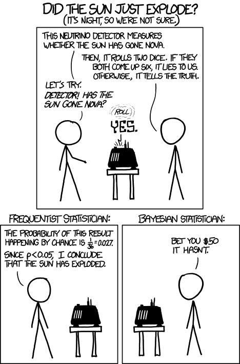
Figure 3. “Frequentists vs. Bayesians,” https://xkcd.com/1132/.
The short answer is — as you go forward do realize that there is a limitation to the frequentist approach and to be on the correct side of the controversy, you need to understand what you can conclude from statistical results. NHST is by far the most commonly used approached in biosciences (eg, out of 49 research articles I checked from four randomly selected issues of 2015 PLoS Biology, 43 used NHST, 2 used a likelihood approach, none used Bayesian statistics). The NHST is also the overwhelming manner in which we teach introductory statistics courses (eg, checking out the various MOOC courses at www.coursera.org, all of the courses related to Basic Statistics or Inferential Statistics are taught primarily from the NHST perspective). However, right from the start I want to emphasize the limits of the NHST approach.
If the purpose of science is to increase knowledge, then the NHST approach by itself is an inadequate framework at best, and in the eyes of some, worthless! Now, I think this latter sentiment is way over the top, but there is a need for us to stop before we begin, in effect, to set the ground rules for what can be interpreted from the NHST approach. The critics of NHST have a very important point, and that needs to be emphasized, but we will also defend use and teaching of this approach so that you are not left with the feeling that somehow this is a waste of time or that you are being cheated from learning the latest knowledge on the subject of statistical inference. The controversy hinges on what probability means.
P-values, statistical power, and replicability of research findings
Science, as a way of knowing how the world works, is the only approach that humans have developed that has been empirically demonstrated to work. Note how I narrowed what science is good for — if we are asking questions about the material world, then science should be your toolkit. Some (eg, Platt 1964), may further argue that there are disciplines in science that have been more successful (eg, molecular biology) than others (eg, evolutionary psychology, cf discussion in Ryle 2006) at advancing our knowledge about the material world. However, to the extent research findings are based solely on statistical results there is reason to believe that many studies in fact have not recovered truth (Ioannidis 2005).
In a review of genomics, it was reported that findings of gene expression differences by many microarray studies were not reproducible (Allison et al 2006). The consensus is that confidence in the findings should hold only for the most abundant gene transcripts of many microarray gene expression profiling studies, a conclusion that undercuts the perceived power of the technology to discover new causes of disease and the basis for individual differences for complex phenotypes. Note that when we write about failure of research reproducibility we are not including cases of alleged fraud (Carlson 2012 on Duke University oncogenomics case), we are instead highlighting that these kinds of studies often lack statistical power; hence, when repeated, the experiments yield different results.
Frequentist and Bayesian Probabilities
Turns out there is a lot of philosophical problems around the idea of “probability,” and three schools of thought. In the Fisherian approach to testing, the researcher devises a null hypothesis, HO, collects the data, then computes a probability (p-value) of the result or outcome of the experiment. If the p-value is small, then this is inferred as little evidence in support of the null hypothesis.
In the Frequentists’ approach, the one we are calling NHST, the researcher devises two hypotheses, the null hypothesis, HO, and an alternative hypothesis, HA. The results are collected from the experiment and, prior to testing, a Type I error rate (α, chance) is defined. The Type I error rate is set to some probability and refers to the chance of rejecting the null hypothesis purely due to random chance. The Frequentist then computes a p-value of result of the experiment and applies a decision criterion: If P-value greater than Type I error rate, then provisionally accept null hypothesis. In both the Fisherian and Frequentist approaches, the probability, again defined at the relative frequency of an event over time, is viewed as a physical, objective and well-defined set of values.
Bayesian approach: based on Bayes conditional probability, one identifies the prior (subjective) probability of an hypothesis, then, adjusts the prior probability (down or up) as new results come in. The adjusted probability is known as posterior probability and it is equal to the likelihood function for the problem. The posterior probability is related to the prior probability and this function can be summarized by the Bayes factor as evidence the evidence against the null hypothesis. And that’s what we want, a metric of our evidence for or against the null hypothesis.
Note 2: A probability distribution function (PDF) is a function of the sample data and returns how likely that particular point will occur in the sample. The distribution is given. The likelihood function approaches this from a different direction. The likelihood function takes the data set as a given and represents how likely are the different parameters for your distribution.
We can calibrate the Bayesian probability to the frequentist p-value (Selke et al 2001; Goodman 2008; Held 2010; Greenland and Poole 2012). Methods to achieve this calibration vary, but the Fagan nomogram Held (2010) proposed is a good tool for us as we go forward. We can calculate our NHST p-value, but then convert the p-value to a Bayes factor by looking at the nomogram. I mention this here not as part of your to do list, but rather as a way past the controversy: the NHST p-value can be interpreted as a Bayesian conditional probability, but they do not test the same hypothesis.
Likelihood
Before we move on there is one more concept to introduce, that of likelihood. We describe a model (an equation) we believe can generate the data we observe. By constructing different models with different parameters (hypotheses), you generate a statistic that yields a likelihood value. If the model fits the data, then the likelihood function has a small value. The basic idea then is to compare related, but different models to see which fits the data better. We will use this approach when comparing linear models when we introduce multiple regression models in Chapter 18.
What’s wrong with the p-value from NHST?
Well, really nothing is “wrong” with the p-value.
Where we tend to get into trouble with the p-value concept is when we try and interpret it. See below, Why is this important to me as a beginning student? The p-value is not evidence for a position, it is a statement about error rates. The p-value from NHST can be viewed as the culmination of a process that is intended to minimize the chance that the statistician makes an error.
In Bayesian terms, the p-value from NHST is the probability that we observe the data (eg, the differences between two sample means), assuming the null hypothesis is true. If we want to interpret the p-value in terms of evidence for a proposition, then we want the conditional error probability.
Sellke et al (2001) provided a calibration of p-values and, assuming that the prior probabilities of the null hypothesis and the alternative hypothesis are equal (that is, that each have a prior probability of 0.5), by using a formula provided by them (equation 3), we can correct our NHST p-value into a probability that can be interpreted as evidence in favor of the interpretation that the null hypothesis is true. In Bayesian terms this is called the posterior probability of the null hypothesis. The formula is

where e is Euler’s number, the base of the natural logarithm (ln), and p is the p-value from the NHST. This calibration works as long as  (Sellke et al 2001).
By convention we set the Type I error at 5% (cf Cohen 1994). How strong of evidence is a p-value near 5% against the null hypothesis being true, again, under the assumption that the prior probability of the null hypothesis being true is 50%? Using the above formula I constructed a plot of the calculated conditional error probability values against p-values (Fig 4).
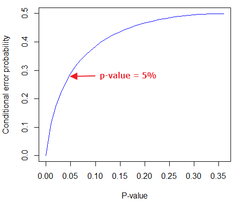
Figure 4. Conditional error probability values plotted against p-values.
As you can see, a p-value of 5% is not strong evidence at just 0.289. Not until p-values are smaller than 0.004 does the conditional error probability value dip below 0.05, suggesting strong evidence against the null hypothesis being true.
R note: For those of you keeping up with the R work, here’s the code for generating this plot. Text after “#” are comments and are not interpreted by R.
At the R prompt type each line
NHSTp = seq(0.00001,0.37,by=0.01)      #create a sequence of numbers between 0.0001 and 0.37 with a step of 0.01
CEP = (1+(-1*exp(1)*NHSTp*log(NHSTp))^-1)^-1    #equation 3 from Sellke et al 2001
plot(NHSTp,CEP,xlab="P-value", ylab="Conditional error probability",type="l",col="blue")
Why is this important to me as a beginning student?
As we go forward I will be making statements about p-values and Type I error rates and null hypotheses and even such things as false positives and false negative. We need to start to grapple with what exactly can be said by p-values in the context of statistical inference, and to recognize that we will sometimes state conclusions that cut some corners when it comes to interpreting p-values. And yet, you (and all consumers of statistics!) are expected to recognize what p-values mean. Always.
The real meaning and interpretation of P-values
This is as good of a time as any to make some clarification about the meaning of p-value and the whole inference concept. Fisher indeed came up with the concept of the p-value, but its use as a decision criterion owes to others and Fisher disagreed strongly with use of the p-value in this way (Fisher 1955; Lehmann 1993).
Here are some common p-value corner-cutting statements to avoid using (after Goodman 2008; Held 2010). P-values are sometimes interpreted, incorrectly, as
Table. Incorrect interpretations of NHST p-values
- the probability of obtaining the observed data under the assumption of no real effect
- an observed type-I error rate
- the false discovery rate, ie, the probability that a significant finding is a “false positive”
- the (posterior) probability of the null hypothesis.
So, if p-values don’t mean any of these things, what does a p-value mean? It means that we begin by assuming that there is no effect of our treatments — the p-value is then the chance we will get as large of a result (our test statistic) and the null hypothesis is true. Note that this definition does not include a statement about evidence of the null hypothesis being true. To get evidence of “truth” we need additional tools, like the Bayes Factor and the correction of the p-value to the conditional error probability (see above). Why not dump all of the NHST and go directly to a Bayesian perspective, as some advise? The single best explanation was embedded in the assumption we made about the prior probability in order to calculate the conditional error probability. We assumed the prior probability was 50%. For many, many experiments, that is simply a guess. The truth is we generally don’t know what the prior probability is. Thus, if this assumption is incorrect, then the justification for the formula by Sellke et al (2001) is weakened, and we are no closer to establishing evidence than before.
The take home message is that it is unlikely that a single experiment will provide strong evidence for the truth. Thus the message is repeat your experiments — and you already knew that! And the Bayesians can tell us that with the addition of more and more data reduces the effect of the particular value of the prior probability on our calculation of the conditional error probability. So, that’s the key to this controversy over the p-value.
Reporting p-values
Estimated p-values can never be zero. Students may come to use software that may return p-values like “0” — I’m looking at you Google Sheets re: default results from CHISQ.TEST() — but again, this does not mean the probability of the result is zero. The software simply reports values to two significant figures and failed to round. Some journals may recommend that 0 should be replaced by p < 0.01 or even < 0.05 inequalities, but the former lacks precision and the latter over-emphasizes the 5% Type I error rate threshold, the “statistical significance” of the result. In general, report p-value to three significant figures and four digits. If a p-value is small, use scientific notation and maintain significant digits. Thus, a p-value of 0.004955794 should be reported as 0.00496 and a p-value of 0.0679 should be reported as 0.0679. Use R’s signif() function, for example p-value reported as 6.334e-05, then
signif(6.334e-05,3)
[1] 6.33e-05
Rounding and significant figures were discussed in Chapter 3.5. See Land and Altman (2015) for guidelines on reporting p-values and other statistical results.
Questions
- Revisit Figure 1 again and consider the following hypothesis — the sun will rise tomorrow.
- If we take the Frequentist position, what would the null hypothesis be?
- If we take the Bayesian approach, identify the prior probability.
- Which approach, Bayesian or Frequentist, is a better approach for testing this hypothesis?
- Consider the pediatrician who, upon receiving a chest X-ray for a child notes the left lung has a large irregular opaque area in the lower quadrant. Based on the X-ray and other patient symptoms, the doctor diagnoses pneumonia and prescribes a broad-spectrum antibiotic. Is the doctor behaving as a Frequentist or a Bayesian?
- With the p-value interpretations listed in the table above in hand, select an article from PLoS Biology, or any of your other favorite research journals, and read how the authors report results of significance testing. Compare the precise wording in the results section against the interpretative phrasing in the discussion section. Do the authors fall into any of the p-value corner-cutting traps?
Quiz Chapter 8.2
The controversy over proper hypothesis testing
Chapter 8 contents
- Introduction
- The null and alternative hypotheses
- The controversy over proper hypothesis testing<.span>
- Sampling distribution and hypothesis testing
- Tails of a test
- One sample t-test
- Confidence limits for the estimate of population mean
- References and suggested readings
7.3 – Conditional Probability and Evidence Based Medicine
- Conditional probability and risk communication
- Probability and independent events
- Example of multiple, independent events
- Probabilistic risk analysis
- Conditional probability of non-independent events
- Diagnosis from testing
- Standard million
- Per capita rate
- Practice and introduce PPV and test decision criteria
- Evidence Based Medicine
- Software
- Example
- Questions
- Quiz
- Chapter 7 contents
Conditional probability and risk communication.
Conditional probabilities can be used to accurately and effectively convey the risk of specific health outcomes to patients and the public. Tools introduced in this chapter help move from an initial assessment of disease risk to a revised probability after a test result is returned. Although there are other interpretations, here we frame EBM — evidence-based-medicine — as a form of Bayesian decision-making.
This sub-chapter covers a lot of ground. We begin by addressing how probability of multiple events are calculated assuming each event is independent. The assumption of independence is then relaxed, and how to determine probability of an event happening given another event has already occurred, conditional probability, is introduced. Use of conditional probability to interpret results of a clinical test are also introduced, along with the concept of EBM. We also introduce Bayes’ rule and Bayesian probability.
Probability and independent events.
Probability distributions are mathematical descriptions of the probabilities of how often different possible outcomes occur. We also introduced basic concepts related to working with the probabilities involving more than one event.
For review, for independent events, you multiply the individual chance that each event occurs to get the overall probability.
Example of multiple, independent events.

Figure 1. Now that’s a box full of kittens. Creative Commons License, source: https://www.flickr.com/photos/83014408@N00/160490011.
What is the chance of five kittens in a litter of five to be of the same sex? In feral cat colonies, siblings in a litter share the same mother, but not necessarily the same father, superfecundation. Singleton births are independent events, thus the probability of the first kitten is female is 50%; the second kitten is female, also 50%; and so on. We can multiply the independent probabilities (hence, the multiplicative rule), to get our answer:
kittens <- c(0.5, 0.5, 0.5, 0.5, 0.5)
prod(kittens)
[1] 0.03125
Probabilistic risk analysis.
Risk analysis is the use of information to identify hazards and to estimate the risk. A more serious example. Consider the 1986 Space Shuttle Challenger Disaster (Hastings 2003). Among the crew killed was Ellison Onizuka, the first Asian American to fly in space (Fig 2, first on left back row). Onizuka was born and raised on Hawai`i and graduated from Konawaena High School in 1964.

Figure 2. STS-51-L crew: (front row) Michael J. Smith, Dick Scobee, Ronald McNair; (back row) Ellison Onizuka, Christa McAuliffe, Gregory Jarvis, Judith Resnik. Image by NASA – NASA Human Space Flight Gallery, Public Domain.
The shuttle was destroyed just 73 seconds after lift off (Fig 3).

Figure 3. Space Shuttle Challenger launches from launchpad 39B Kennedy Space Center, FL, at the start of STS-51-L. Hundreds of shorebirds in flight. Image by NASA – NASA Human Space Flight Gallery, Public Domain.
This next section relies on material and analysis presented in the Rogers Commission Report June 1986. NASA had estimated that the probability of one engine failure would be 1 in 100 or 0.01; two engine failures would mean the shuttle would be lost. Thus, the probability of two rockets failing at the same time was calculated as 0.01 X 0.01, which is 0.0001 or 0.01%.
NASA had planned to fly the fleet of shuttles 100 times per year, which would translate to a shuttle failure once in 100 years. The Challenger launch on January 28, 1986, represented only the 25th flight of the shuttle fleet.
One difference on launch day was that the air temperature at Cape Canaveral was quite low for that time of year, as low as 22 °F overnight.
Attention was pointed at the large O-rings in the boosters (engines). In all, there were six of these O-rings. Testing suggested that, at the colder air temperatures, the chance that one of the rings would fail was 0.023. Thus, the chance of success was only 0.977. Assuming independence, what is the chance that the shuttle would experience O-ring failure?
shuttle <- c(0.977, 0.977, 0.977, 0.977, 0.977, 0.977)
#probability of success then was
prod(shuttle)
[1] 0.869

#and therefore probability of failure was
1 - prod(shuttle)
[1] 0.1303042
Conditional probability of non-independent events.
But in many other cases, independence of events cannot be assumed. The probability of an event given that another event has occurred is referred to as conditional probability. Conditional probability is used extensively to convey risk. We’ve touched on some of these examples already:
- the risk of subsequent coronary events given high cholesterol;
- the risk of lung cancer given a person smokes tobacco;
- the risk of mortality from breast cancer given that regular mammography screening was conducted.
There are many, many examples in medicine, insurance, you name it. It is even an important concept that judges and lawyers need to be able to handle (eg, discussion in Berry 2008).
A trigger warning: what follows is emotional, traumatic material, provided to emphasize the importance of these concepts, and the far-reaching implications understanding conditional probability can have for us.
A now famous example of conditional probability in the legal arena came from arguments over the chance that a husband or partner who beats his wife will subsequently murder her — this was an argument raised by the prosecution during pre-trial in the 1995 O.J. Simpson trial (The People of the State of California v. Orenthal James Simpson), and successfully argued by O.J. Simpson’s attorneys… judge ruled in favor of the defense and evidence of O.J. Simpson’s prior abuse were not included in trial. Gigerenzer (2002, following discussions by others, eg, Good 1995) and others (eg, Skorupski and Wainer 2015), have called this the Defendent’s Fallacy, the reverse of the Prosecutor’s Fallacy, where the more typical scenario is that the prosecution provides a list of probabilities about characteristics of the defendant, leaving the jury to conclude that no one else could have possibly fit the description ( and 1987).
In the O.J. Simpson case, the argument went something like this. From the CDC we find that the chance of an average woman being murdered by a stranger or an unrelated party was about 1 in 20,000. CDC statistics indicate 1.3 million women are abused each year by their partner or former partner; each year about 1000 women are murdered. One thousand divided by 1.3 million is a small number, so even when there is abuse the argument goes, 99% of the time there is not murder. The Simpson judge ruled in favor of the defense and much of the evidence of prior abuse was excluded.
Something is missing from the defense’s argument. Nicole Brown Simpson did not belong to a population of battered women — she belonged to the population of murdered women. When we ask, if a woman is murdered, what is the chance that she knew her murderer, we find that more than 55% knew their murderer — and of that 55%, 93% were killed by a partner who had a history of prior abuse against the victim.
Instead of looking at all 1.3 million abused women, we isolate a representative cohort of 100,000 abused women to see what mathematically happens to them in a given year:
Group 1: Murdered by their abuser. According to the defense’s rate of 1 in 2,500:
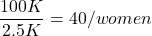
Group 2: Murdered by someone else:
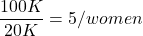
Given that an abused woman was murdered, what is the probability it was done by her abuser?

or 89%.
This is a huge difference from how the Defense portrayed the chance, where they wanted the judge to assume every single one of those 2500 abusers is equally likely to have committed the crime. In reality, we must condition the match on all other available evidence.
The key — Nicole Simpson (and Ron Goldman) were murdered; O.J. Simpson was an ex-partner who had been guilty of assault against Nicole Simpson. Now, it goes from an impossibly small chance, to a much greater chance. Conditional probability, and specifically Bayes’ rule, is used for these kinds of problems. The defense successfully masked a probability that was heavily stacked against their client.
Bayes’ rule provides guidance for how to update the probability of an event based on new evidence. Named after Thomas Bayes (1701- 1761), more generally, Bayes’ rule, described below, is used to quantify conditional probability. Bayesian probability, where probability is interpreted as reasonably expectation instead of frequency of some event. We discuss Bayesian and Frequentist approaches to hypothesis testing in Chapter 8.2.
Note 1: Following our epidemilogy definitions, women murdered by their abuser (Group 2), epidemiology terms, that would be  , the exposure rate in controls, whereas abused woman murdered by her abuser (Group 1), that would be
 , the exposure rate in cases.
Diagnosis from testing.
Let’s turn our attention to medicine. A growing practice in medicine is to claim that decision making in medicine should be based on approaches that give us the best decisions. A search of PubMed texts for “evidence based medicine” found more than 91,944 (13 October 2021, and increase of thirteen thousand since last I looked (10 October, 2019). Evidence based medicine (EBM) is the “conscientious, explicit, judicious and reasonable use of modern, best evidence in making decisions about the care of individual patients” (Masic et al 2008). By evidence, we may mean results from quantitative, systematic reviews, meta-analysis, of research on a topic of medical interest, eg, Cochrane Reviews.
Note 2: Primary research refers to generating or collecting original data in pursuit of tests of hypotheses. Both systematic reviews and meta-analysis are secondary research or “research on research.” As opposed to a literature review, systematic review make explicit how studies were searched for and included; if enough reasonably similar quantitative data are obtained through this process, the reviewer can combine the data and conduct an analysis to assess whether a treatment is effective (De Vries 2018).
As you know, no diagnostic test is 100% fool-proof. For many reasons, test results come back positive when the person truly does not have the condition — this is a false positive result. Correctly identifying individuals who do not have the condition, 100% – false positive rate, is called the specificity of a test.
Think of specificity in this way — provide the test 100 true negative samples (eg, 100 samples from people who do not have cancer) — how many times out of 100 does the test correctly return a “negative”? If 99 times out of 100, then the specificity rate for this test is 99%. Which is pretty good. But the test results mean more if the condition/disease is common; for rare conditions, even 99% is not good enough. Incorrect assignments are rare, we believe, in part because the tests are generally quite accurate. However, what we don’t consider is that detection and diagnosis from tests also depend on the base rate — how frequent the incidence of the condition is in the population. Paradoxically, the lower the base rate, the poorer diagnostic value even a sensitive test may have.
Note 3: This concept, that the base rate effects clinical relevance of interpreting testing — has really important, real-world consequences. It directly bears on clinical testing of cancer and other relatively rare diseases; it also dramatically influences applicability of highly sensitive tests for drug use in clinical samples.
To summarize our jargon for interpreting a test or assay, so far we have
- True positive (a), the person has a disease and the test correctly identifies the person as having the disease.
- False positive (b), test result incorrectly identifies disease; the person does not have the disease, but the test classifies the person as having the disease.
- False negative (c), test result incorrectly classifies person does not have disease, but the person actually has the disease.
- True negative (d), the person does not have the disease and the test correctly categorizes the person as not having the disease.
- Positive predictive value (PPV), the proportion of patients with a positive test result who actually have the disease,
 .
- Negative Predictive Value (NPV), the probability that a person who receives a negative test result really does not have the disease,
 .
- Negative Predictive Value (NPV), the probability that a person who receives a negative test result really does not have the disease,
- Sensitivity of test (Se), the proportion of persons who test positive and do have the disease (true positives):
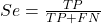
If a test has 75% sensitivity, then out of 100 individuals who do have the disease, then 75 will test positive (TP = true positive). - Specificity of a test (Sp), refers to the rate that a test correctly classifies a person that does not have the disease (TN = true negatives):
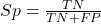
If a test has 90% specificity, then out of 100 individuals who truly do not have the disease, then 90 will test negative (= true negatives).
A worked example. A 50 year old male patient is in the doctor’s office. The doctor is reviewing results from a diagnostic test, eg, a FOBT — fecal occult blood test — a test used as a screening tool for colorectal cancer (CRC). The doctor knows that the test has a sensitivity of about 75% and specificity of about 90%. Prevalence of CRC in this age group is about 0.2% (cf NCI SEER). The prevalence is also the prior probability — the baseline rate of the condition in the population before a test is taken. Figure 4 shows our probability tree using our natural numbers approach (Fig 4).
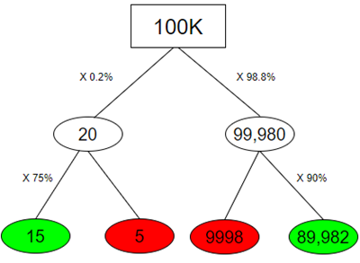
Figure 4. Probability tree for FOBT test; Good test outcomes shown in green: TP stands for true positive and TN stands for true negative. Poor outcomes of a test shown in red: FN stands for false negative and FP stands for false positive.
Note 4: Since U.S. Preventative Task Force (2021), FOBT has largely been replaced by Fecal Immunochemical Test (FIT): sensitivity 74%, specificity 95%, and Multitarget Stool DNA Test: sensitivity 76%, specificity 90%. Cologuard combines both: sensitivity 92%, specificity 97% (cf discussion in Imperiale et al 2014).
- The U.S. Supreme Court (Kennedy v. Braidwood Management, Inc) supported USPSTF’s authority to recommend preventive services covered by insurers (see 2025 article by R. Payerchin in Medical Economics).
The associated probabilities for the four possible outcomes of these kinds of tests (eg, what’s the probability of a person who has tested positive in screening tests actually has the disease?) are shown in Table 1.
Table 1. A 2 X 2 table of possible outcomes of a diagnostic test.
| Person really has the disease | ||
| Test Result | Yes | No |
| Positive | a TP |
b FP |
| Negative | c FN |
d TN |
We want the posterior probability — the chance that a positive test result is a true positive. Bayes’ rule is often given in probabilities,

Bayes’ rule, where truth is represented by either D (the person really does have the disease”) or ND (the person really does not have the disease”) and ⊕ is symbol for “exclusive or” and reads “not D” in this example.
An easier way to see this is to use frequencies and our table instead (Table 1, numbers in Figure 4).
Now, the formula is

Simplified Bayes’ rule, where a is the number of people who test positive and DO HAVE the disease and b is the number of people who test positive and DO NOT have the disease. Thus,  , the posterior probability was

or 0.15%. Because the condition is so rare (0.2% prior) and the test generates a very high number of False Positives (9,998), getting a positive result actually lowers oour confidence slightly from the base rate (from 0.2% down to 0.15%). This occurs because the test is highly unreliable in screening this specific population — it’s known as the base rate fallacy. Thus, the chance that a positive FOBT test for our 50 year old male patient is 99.85% likely wrong.
Standardized million.
Where did the 100,000 come from? We discussed this in chapter 2: it’s a simple trick to adjust rates to the same population size. We use this to work with natural numbers instead of percent or frequencies. You choose to correct to a standardized population based on the raw incidence rate. A rough rule of thumb:
Table 2. Relationship between standard population size and incidence rate.
| Raw IR rate about | IR | Standard population |
| 1/10 | 10% | 1000 |
| 1/100 | 1% | 10,000 |
| 1/1000 | 0.1% | 100,000 |
| 1/10,000 | 0.01% | 1,000,000 |
| 1/100,000 | 0.001% | 10,000,000 |
| 1/1,000,000 | 0.0001% | 100,000,000 |
The raw incident rate is simply the number of new cases divided by the total population.
Per capita rate.
Yet another standard manipulation is to consider the average incidence per person, or per capita rate. The Latin “per capita” translates to “by head” (Google translate), but in economics, epidemiology, and other fields it is used to reflect rates per person. Tuberculosis is a serious infectious disease of primarily the lungs. Incidence rates of tuberculosis in the United States have trended down since the mid 1900s: 52.6 per 100K in 1953 to 2.7 per 100K in 2019 (CDC). Corresponding per capita values are 5.26 x 10⁻⁴ and 2.7 x 10⁻⁵, respectively. Divide the rate by 100,000 to get per person rate.
Practice and introduce PPV and test decision criteria.
Let’s break these problems down, and in doing so, introduce some terminology common to the field of “risk analysis” as it pertains to evaluating assay and diagnotistc tests in biology and epidemiology. Our first example considers the fecal occult blood test, FOBT, test. Blood in the stool may (or may not) indicate polys or colon cancer (Park et al 2010).
A table like the one shown above (Table 1) will appear again and again throughout this and subsequent chapters, but in different forms. We start with Table 3.
Table 3. A 2 X 2 table of possible outcomes of FOBT test.
| Person really has the disease | |||
| Yes | No | ||
| Positive | 15 | 9998 | PPV = 15/(15+9998) = 0.15% |
| Negative | 5 | 89,982 | NPV = 89982/(89982+5) = 99.99% |
We want to know how good is the test, particularly if the goal is early detection? This is conveyed by the PPV, positive predictive value of the test. Unfortunately, the prevalence of a condition is also at play: the lower the prevalence, the lower the PPV must be, because most positive tests will be false when population prevalence is low.
Youden (1950) proposed a now widely adopted index that summarizes how effective a test is. Youden’s J is the sum of specificity and sensitivity minus one.

where Se stands for sensitivity of the test and Sp stands for sensitivity of the test.
Youden’s J takes on values between 0, for a terrible test, and 1, for a perfect test. For our FOBT example, Youden’s J was 0.65. This statistic looks like it’s independent of prevalence, but it’s use as a decision criterion (eg, a cutoff value, above which test is positive, below test is considered negative), assumes that the cost of misclassification (false positives, false negatives) are equal. Prevalence affects number of false positives and false negatives for a given diagnostic test, so any decision criterion based on Youden’s J will also be influenced by prevalence (Smits 2010).
Youden’s J is insensitive to base rates and therefore may be of little practical use in the field. Unsurprisingly, other tools are available, including Matthew’s Correlation Coefficient (MCC),

and the positive and negtive Clinical Utility Index (CUI+, CUI-),

or the F1-score,

epiR will calculate Youden’s J, but the others are either calculated by hand or by way of additional packages. So, we’ll provide a function.
R code to calculate testing decision criteria — code genereated with Gemini AI assistance.
run_screening_wizard <- function() {
# 1. Sequential user prompts starting with cell a
cat("--- 2x2 Matrix Entry Wizard ---\n")
a <- as.numeric(readline(prompt = "Enter cell a (True Positives, TP): "))
b <- as.numeric(readline(prompt = "Enter cell b (False Positives, FP): "))
c <- as.numeric(readline(prompt = "Enter cell c (False Negatives, FN): "))
d <- as.numeric(readline(prompt = "Enter cell d (True Negatives, TN): "))

# 2. Map cells to short variables for calculation
tp <- a
fp <- b
fn <- c
tn <- d

# 3. Construct and print the visual 2x2 matrix
user_matrix <- matrix(
c(tp, fp, fn, tn),
nrow = 2,
byrow = TRUE,
dimnames = list(Test = c("+", "-"), Disease = c("+", "-"))
)
cat("\n[+] Captured Matrix:\n")
print(user_matrix)

# 4. Run background metrics math
sensitivity <- tp / (tp + fn)
specificity <- tn / (tn + fp)
ppv <- tp / (tp + fp)
if (is.nan(ppv)) ppv <- 0

youden_j <- sensitivity + specificity - 1
cui_pos <- sensitivity * ppv

f1_score <- 2 * ((ppv * sensitivity) / (ppv + sensitivity))
if (is.nan(f1_score)) f1_score <- 0

mcc_num <- (tp * tn) - (fp * fn)
mcc_den <- sqrt(as.numeric(tp + fp) * as.numeric(tp + fn) *
as.numeric(tn + fp) * as.numeric(tn + fn))
mcc <- if (mcc_den == 0) 0 else mcc_num / mcc_den

# 5. Compile into the copy/paste ready console matrix
output_matrix <- matrix(
c(round(youden_j, 4), "No", "Good (Overly optimistic baseline)",
round(mcc, 4), "Yes", "Poor (Correctly captures imbalance)",
round(cui_pos, 4), "Yes", "Unacceptable clinical utility",
round(f1_score, 4), "Yes", "Near-total prediction failure"),
nrow = 4, byrow = TRUE
)

dimnames(output_matrix) <- list(
c("Youden's J Index", "MCC", "CUI+", "F1-Score"),
c("Value", "Base_Rate_Dep", "Console_Interpretation")
)

final_df <- as.data.frame(output_matrix)

# 6. Print and invisibly return the dataframe
cat("\n[+] Resulting Metrics Table (Copy/Paste Ready):\n")
print(final_df)
return(invisible(final_df))
}

# Run the function at the R command prompt.
run_screening_wizard()
End R code.
Thus, using a metric sensitive to low base rate, our FOBT tests are (modified from R output)
Table 4. Decision criteria.
| Value | Base rate dependent? | Interpretation | |
 |
0.65 | No | Good |
 |
0.0306 | Yes | Poor |
 |
0.0011 | Yes | Unacceptable clinical utility |
 |
0.0030 | Yes | Near-total prediction failure |
Another worked example. A study on cholesterol-lowering drugs (statins) reported a relative risk reduction of death from cardiac event by 22%. This does not mean that for every 1000 people fitting the population studied, 220 people would be spared from having a heart attack. In the study, the death rate per 1000 people was 32 for the statin versus 41 for the placebo — recall that a placebo is a control treatment offered to overcome potential patient psychological bias (see Chapter 5.4). The absolute risk reduction due to statin is only 41 – 32 or 9 in 1000 or 0.9%. By contrast, relative risk reduction is calculated as the ratio of the absolute risk reduction (9) divided by the proportion of patients who died without treatment (41), which is 22% (LIPID Study Group 1998).
Note that risk reduction is often conveyed as a relative rather than as an absolute number. The distinction is important for understanding arguments based in conditional probability. Thus, the question we want to ask about a test is summarized by absolute risk reduction (ARR) and number needed to treat (NNT), and for problems that include control subjects, relative risk reduction (RRR). We expand on these topics in the next section, 7.4 – Epidemiology: Relative risk and absolute risk, explained.
Evidence Based Medicine.
One culture change in medicine is the explicit intent to make decisions based on evidence (Masic et al 2008). Of course, the joke then is, well, what were doctors doing before, diagnosing without evidence? The comic strip xkcd offers one possible answer (Fig 5).
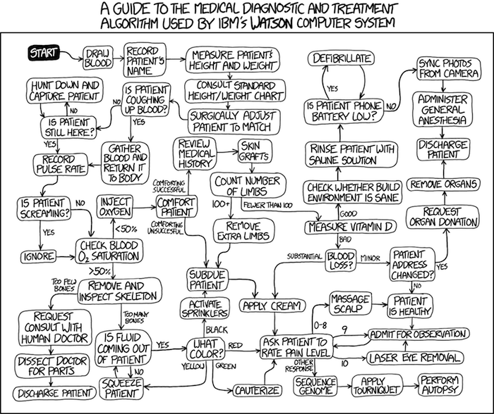
Figure 5. A summary of “evidence based medical” decisions, perhaps? “Watson Medical Algorithm,” https://xkcd.com/1619/.
As you can imagine, there’s considerable reflection about the EBM movement (see discussions in response to Accad and Francis 2018, eg, Goh 2018). More practically, our objective is for you to be able to work your way through word problems involving risk analysis. You can expect to be asked to calculate, or at least set up for calculation, any of the statistics listed above (eg, False negative, false positive, etc.). Practice problems are listed at the end of this section, and additional problems are provided to you (Homework 4). You’ll also want to check your work, and in any real analysis, you’d most likely want to use R.
Software.
R has several epidemiology packages, and with some effort, can save you time. Another option is to run your problems in OpenEpi, a browser-based set of tools. OpenEpi is discussed with examples in the next section, 7.4.
Here, we illustrate some capabilities of the epiR package, expanded more also in the next section, 7.4. We’ll use the example from Table 3.
R code
library(epiR)
Table3 <- matrix(c(15, 5, 9998, 89982), nrow = 2, ncol = 2)
epi.tests(Table3)
R output
         Outcome + Outcome -   Total
Test +          15      9998   10013
Test -           5     89982   89987
Total           20     99980  100000

Point estimates and 95% CIs:
--------------------------------------------------------------
Apparent prevalence *                      0.10 (0.10, 0.10)
True prevalence *                          0.00 (0.00, 0.00)
Sensitivity *                              0.75 (0.51, 0.91)
Specificity *                              0.90 (0.90, 0.90)
Positive predictive value *                0.00 (0.00, 0.00)
Negative predictive value *                1.00 (1.00, 1.00)
Positive likelihood ratio                  7.50 (5.82, 9.67)
Negative likelihood ratio                  0.28 (0.13, 0.59)
False T+ proportion for true D- *          0.10 (0.10, 0.10)
False T- proportion for true D+ *          0.25 (0.09, 0.49)
False T+ proportion for T+ *               1.00 (1.00, 1.00)
False T- proportion for T- *               0.00 (0.00, 0.00)
Correctly classified proportion *          0.90 (0.90, 0.90)
--------------------------------------------------------------
* Exact CIs
Oops! I wanted PPV, which by hand calculation was 0.15%, but R reported “0.00?” This is a significant figure reporting issue. The simplest solution is to submit options(digits=6) before the command, then save the output from epi.tests() to an object and use summary(). For example
options(digits=6)
myEpi <- epi.tests(Table3)
summary(myEpi)
And R returns
     statistic           est        lower        upper
1           ap  0.1001300000 0.0982761568  0.102007072
2           tp  0.0002000000 0.0001221693  0.000308867
3           se  0.7500000000 0.5089541283  0.913428531
4           sp  0.9000000000 0.8981238085  0.901852950
5      diag.ac  0.8999700000 0.8980937508  0.901823014
6      diag.or 27.0000000000 9.8110071871 74.304297826
7         nndx  1.5384615385 1.2265702376  2.456532054
8       youden  0.6500000000 0.4070779368  0.815281481
9       pv.pos  0.0014980525 0.0008386834  0.002469608
10      pv.neg  0.9999444364 0.9998703379  0.999981958
11      lr.pos  7.5000000000 5.8193604069  9.666010707
12      lr.neg  0.2777777778 0.1300251423  0.593427490
13      p.rout  0.8998700000 0.8979929278  0.901723843
14       p.rin  0.1001300000 0.0982761568  0.102007072
15      p.tpdn  0.1000000000 0.0981470498  0.101876192
16      p.tndp  0.2500000000 0.0865714691  0.491045872
17      p.dntp  0.9985019475 0.9975303919  0.999161317
18      p.dptn  0.0000555636 0.0000180416  0.000129662
There we go — pv.pos reported as 0.0014980525, which, after turning to a percent and rounding, we have 0.15%. Note also the additional statistics provided — a good rule of thumb — always try to save the output to an object, then view the object, eg, with summary(). Refer to help pages for additional details of the output (?epi.tests).
What about R Commander menus?
Note 3: Confirmed Fall 2026 — I have not been able to run the EBM plugin successfully! Simply returns an error message — — on data sets which have in the past performed perfectly. Thus, until further notice, do not use the EBM plugin. Instead, use commands in the epiR package. I’m leaving the text here on the chance the error with the plugin is fixed.
Rcmdr has a plugin that will calculate ARR, RRR and NNT. The plugin is called RcmdrPlugin.EBM (Leucuta et al 2014) and it would be downloaded as for any other package via R.
Download the package from your selected R mirror site, then start R Commander.
install.packages("RcmdrPlugin.EBM")
From within R Commander (Fig 6), select
Tools → Load Rcmdr plug-in(s)…
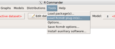
Figure 6. To install an Rcmdr plugin, first go to Rcmdr → Tools → Load Rcmdr plug-in(s)…
Next, select from the list the plug-in you want to load into memory, in this case, RcmdrPlugin.EBM (Fig 7).
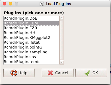
Figure 7. Select the Rcmdr plugin, then click the “OK” button to proceed.
Restart Rcmdr again (Fig 8),
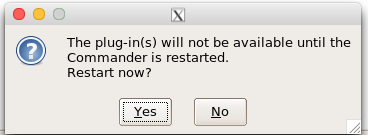
Figure 8. Select “Yes” to restart R Commander and finish installation of the plug-in.
and the menu “EBM” should be visible in the menu bar (Fig 9).
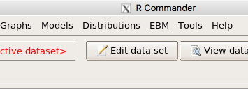
Figure 9. After restart of R Commander the EBM plug-in is now visible in the menu.
Note that you will need to repeat these steps each time you wish to work with a plug-in, unless you modify your .RProfile file. See
Rcmdr → Tools → Save Rcmdr options…
Clicking on the EBM menu item brings up the template for the Evidence Based Medicine module. We’ll mostly work with 2 X 2 tables (eg, see Table 1) , so select the “Enter two-way table…” option to proceed (Fig 10).
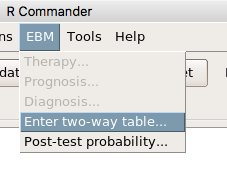
Figure 10. Select “Enter two-way table…”.
And finally, Figure 11 shows the two-way table entry cells along with options. We’ll try a problem by hand then use the EBM plugin to confirm and gain additional insight.
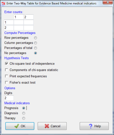
Figure 11. Two-way table Rcmdr EBM plug-in.
For assessing how good a test or assay is, use the Diagnosis option in the EBM plugin. For situations with treated and control groups, use Therapy option. For situations in which you are comparing exposure groups (eg, smokers vs non-smokers), use the Prognosis option.
Example.
Here’s a simple one (problem from Gigerenzer 2002).
About 0.01% of men in Germany with no known risk factors are currently infected with HIV. If a man from this population actually has the disease, there is a 99.9% chance the tests will be positive. If a man from this population is not infected, there is a 99.9% chance that the test will be negative. What is the chance that a man who tests positive actually has the disease?
Start with the reference, or base population (Figure 12). It’s easy to determine the rate of HIV infection in the population if you use numbers. For 10,000 men in this group, exactly one man is likely to have HIV (0.0001X10,000), whereas 9,999 would not be infected.
For the man who has the disease it’s virtually certain that his results will be positive for the virus (because the sensitivity rate = 99.9%). For the other 9,999 men, one will test positive (the false positive rate = 1 – specificity rate = 0.01%).
Thus, for this population of men, for every two who test positive, one has the disease and one does not, so the probability even given a positive test is only 100*1/2 = 50%. This would also be the test’s Positive Predictive Value.
Note that if the base rate changes, then the final answer changes! For example, if the base rate was 10%
It also helps to draw a tree to help you determine the numbers (Fig 12)
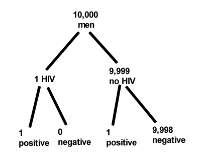
Figure 12. Draw a probability tree to help with the frequencies.
From our probability tree in Figure 12 it is straight-forward to collect the information we need.
- Given this population, how many are expected to have HIV? Two.
- Given the specificity and sensitivity of the assay for HIV, how many persons from this population will test positive? Two.
- For every positive test result, how many men from this population will actually have HIV? One.
Thus, given this population with the known risk associated, the probability that a man testing positive actually has HIV is 50% (=1/(1+1)).
Use the EBM plugin. Select two-way table, then enter the values as shown in Fig 13.
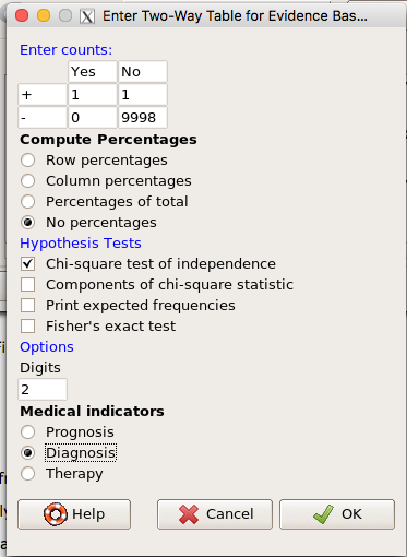
Figure 13. EBM plugin with data entry.
Select the “Diagnosis” option — we are answering the question: How probable is a positive result given information about sensitivity and specificity of a diagnosis test. The results from the EBM functions are given below
Rcmdr> .Table
      Yes No
   +  1    1
   -  0 9998
Rcmdr> fncEBMCrossTab(.table=.Table, .x='', .y='', .ylab='', .xlab='',
Rcmdr+ .percents='none', .chisq='1', .expected='0', .chisqComp='0', .fisher='0',
Rcmdr+ .indicators='dg', .decimals=2)
# Notations for calculations
        Disease + Disease -
Test +      "a"         "b"
Test -      "c"         "d"
# Sensitivity (Se) = 100 (95% CI 2.5 - 100) %. Computed using formula: a / (a + c)
# Specificity (Sp) = 99.99 (95% CI 99.94 - 100) %. Computed using formula: d / (b + d)
# Diagnostic accuracy (% of all correct results) = 99.99 (95% CI 99.94 - 100) %. Computed using formula: (a + d) / (a + b + c + d)
# Youden's index = 1 (95% CI 0.02 - 1). Computed using formula: Se + Sp - 1
# Likelihood ratio of a positive test = 9999 (95% CI 1408.63 - 70976.66). Computed using formula: Se / (Sp - 1)
# Likelihood ratio of a negative test = 0 (95% CI 0 - NaN). Computed using formula: (1 - Se) / Sp
# Positive predictive value = 50 (95% CI 1.26 - 98.74) %. Computed using formula: a / (a + b)
# Negative predictive value = 100 (95% CI 99.96 - 100) %. Computed using formula: d / (c + d)
# Number needed to diagnose = 1 (95% CI 1 - 40.91). Computed using formula: 1 / [Se - (1 - Sp)]
Note that the formulas used to calculate Sensitivity, Specificity, etc., follow our Table 1 (compare to “Notations for calculations”). The use of EBM provides calculations of our confidence intervals.
Questions.
- The sensitivity of the fecal occult blood test (FOBT) is reported to be 0.68. What is the False Negative Rate?
- The specificity of the fecal occult blood test (FOBT) is reported to be 0.98. What is the False Positive Rate?
- For men between 50 and 54 years of age, the rate of colon cancer is 61 per 100,000. If the false negative rate of the fecal occult blood test (FOBT) is 10%, how many persons who have colon cancer will test negative?
- For men between 50 and 54 years of age, the rate of colon cancer is 61 per 100,000. If the false positive rate of the fecal occult blood test (FOBT) is 10%, how many persons who do not have colon cancer will test positive?
- A study was conducted to see if mammograms reduced mortality
Mammogram Deaths/1000 women No 4 Yes 3 data from Table 5-1 p. 60 Gigerenzer (2002)
What is the RRR? - A study was conducted to see if mammograms reduced mortality
Mammogram Deaths/1000 women No 4 Yes 3 data from Table 5-1 p. 60 Gigerenzer (2002)
What is the NNT? - Does supplemental Vitamin C decrease risk of stroke in Type II diabetic women? A study conducted on 1923 women, a total of 57 women had a stroke, 14 in the normal Vitamin C level and 32 in the high Vitamin C level. What is the NNT between normal and high supplemental Vitamin C groups?
- Sensitivity of a test is defined as
A. False Positive Rate
B. True Positive Rate
C. False Negative Rate
D. True Negative Rate - Specificity of a test is defined as
A. False Positive Rate
B. True Positive Rate
C. False Negative Rate
D. True Negative Rate - In thinking about the results of a test of a null hypothesis, Type I error rate is equivalent to
A. False Positive Rate
B. True Positive Rate
C. False Negative Rate
D. True Negative Rate - During the Covid-19 pandemic, number of reported cases each day were published. For example, 155 cases were reported for 9 October 2020 by Department of Health. What is the raw incident rate?
Quiz Chapter 7.3
Conditional Probability and Evidence Based Medicine
Chapter 7 contents
- Introduction
- Epidemiology definitions
- Epidemiology basics
- Conditional Probability and Evidence Based Medicine
- Epidemiology: Relative risk and absolute risk, explained
- Odds ratio
- Confidence intervals
- References and suggested readings
2.6 – Statistical reasoning
How statistical reasoning helps us spot and reduce bias.
.
So far in the course we have talked about statistical reasoning. Statistical reasoning as part of the critical thinking tool kit. What this should mean for you in practice is that we will be developing and enhancing your critical thinking skill set. Here, we’ll define our terms and place statistical reasoning in context.
Critical thinking.
.
What do I mean by critical thinking? You’ll find various definitions and discussions, but the Wikipedia entry on the subject seems as good a start as anything else I have heard or read:
“Critical thinking is a way of deciding whether a claim is always true, sometimes true, partly true, or false” (5 August 2013, http://en.wikipedia.org/wiki/Critical_thinking).
Which raises the question, what is truth (false)? And what about the frequency qualifiers “always,” “sometimes,” “partly”? This hints at one of the strengths of science; “Truth in science … is never final, and what is accepted as fact today may be modified or even discarded tomorrow” (p. 2, National Academy of Science 1999). Scientists extend and even correct the work of their predecessors.
Critical thinking has many definitions, but they coalesce broadly as the search for rational justification — arguments and decisions based on reason not emotion — given sets of facts. We’ll define facts as assertions about the world that are verifiably true. Related to facts, we define evidence as collection of facts used to infer an assertion or belief is objectively true. Objectivity holds independently of the observer. In practice, critical thinking can be improved by identifying and developing certain skill sets, from deductive reasoning to use of a statistical toolkit, although skills alone do not necessarily lead to sound critical thinking (Bailin 2002). Emphasis on the importance of statistical reasoning, for example in the Evidence-Based Medicine (EBM) approach, is now well established. EBM is an expansive concept, but includes the philosophy that decisions in medicine and health care should be based on evidence (results) from well designed and executed research. More generally, much has been written on the subject. My purpose here is to sell you just a bit that you will learn more than formulas and statistical tests in this course; if we do this right you will improve your critical thinking skills.
And the tool kit for critical thinking? Science has the scientific method to offer. In turn, by adopting statistical reasoning approaches you will be more cognizant of whether or not you are indeed engaged in critical thinking about your work.
A working checklist for critical evaluation of a project
- “All sides” of the problem are fairly represented
- Authority is not synonymous with empirical truth: trust, but verify
- Correlation (association) may or may not infer causation
- Do conflicts of interest compromise conclusions?
In other words, identify and rigorously consider assumptions made to reach conclusions, evidence given in support of conclusions, and considerations of bias held by the researcher. The “all sides” part requires judgement — not all sides of a research question are equally valid; the point about “fair” representation requires that opposing arguments are actually held by others and not simply a “”straw man” characterization of of a position held by no one.
Rigid adherence to “how to do science checklist” is likely to be wanting and thus practicing and successful scientists show more flexibility. And, the list is certainly incomplete because it presumes observations and data collection are from a reliable, unbiased source. Before proceeding with how statistics informs our critical thinking in science, let’s illustrate bias.
Bias everywhere.
.
Bias is defined as any tendency that may hamper our ability to answer a question without prejudice (Pannucci and Wilkins 2010). Although we tend to think of ourselves as highly rational (Note 1), psychologists have documented, named numerous, and in some cases, highly specific kinds of cognitive biases we may have about “real world data” that may impair our judgment about results of experiments.
Note 1. A handful of Nobel prizes were awarded over evidence and theory on just how unrational we are, see Simon (1978), Kahneman (2002), and Thaler (2017, whose views were immortalized in the movie The Big Short).
At its best, application of the scientific method is our best tool kit to help protect our conclusions against bias (Nuzzo 2015), by proper experimental design and possible study biases. A couple of comics from xkcd illustrate.
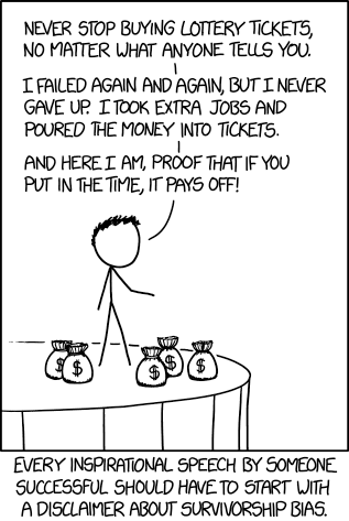
Figure 1. “Survivorship bias,” https://www.xkcd.com/1827/ .
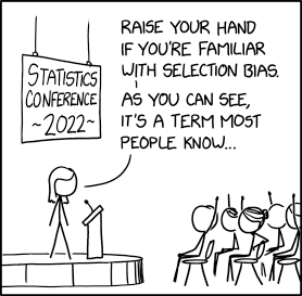
Figure 2. “Selection bias,” https://xkcd.com/2618/ .
Wikipedia lists dozens of named biases which may influence our ability to interpret science:
- confirmation bias, eg, given extraneous information about ancestry or sex, forensic investigators were more likely to assign ancestry or sex of skeletal evidence to group that confirmed the contextual information (Nakhaeizadeh et al 2014).
- congruence bias, a type of confirmation bias, the tendency to test only a favorite or initial hypothesis over consideration of alternative hypotheses.
- observer-expectancy bias, eg, randomized controlled trials of acupuncture often find equivalent responses to real and placebo acupuncture despite both appearing superior to no treatment (Colagiuri and Smith 2012).
- selection bias, the selection of individuals, groups, or data for analysis in such a way that proper randomization is not achieved, eg, mitotic counts (Cree et al 2021) and cell differentials and Figure 2. Selection bias, where the study population is not well-defined or if is, the method by which subjects are recruited favors one kind of subject over another.
- surveillance bias, eg, association between myocarditis and COVID-19 vaccines may be due to increased focus to identify myocarditis (Husby et al 2021).
- survivorship bias, focusing on subjects that passed a selection process as if they represent an entire group, eg, from ecology: rare species more likely to go extinct than abundant species (Lockwood 2003) and Figure 1.
Bias in research may occur at any level, from study design to analysis and publication of results. Bias leads to systematic errors that may favor one outcome over others. Clearly then, bias is something one wants to avoid in science, and most scientists would probably agree strongly that bias is unacceptable. However, bias can creep into projects in many forms.
Particularly pernicious causes of bias are conflicts of interest, with the notable case of a 1990’s set of trials in gene therapy (Wilson 2010). Biased research may be more harmful to science than deliberate misconduct, at least in part because there are, or should be, mechanisms to detect fraud (eg, Marusic et al 2007). If errors in data analysis or management are rare, we can trust the results; if errors are common, systematic, or deliberate falsification, then any conclusions drawn from such work deserves retraction at the very least (cf. discussion in Baggerly and Coombs 2009; see StatCheck project, Nuijten et al 12016).
Bias in research.
.
Bias is not limited to obvious profit seeking or even defense of one’s ideas or reputation. Bias can enter research in subtle ways. Prior to 2000, many post-menopausal women could expect to be placed on hormone replacement therapy (HRT) to manage post-menopausal symptoms and to reduce likelihood of osteoporosis later in life. Moreover, HRT was believed based on research to show protective benefits against heart disease (eg, Nabulsi et al 1993; Grodstein et al 2000). However, other prospective studies that were designed to reduce many sources of bias in patient recruitment (Women’s Health Initiative Study Group 1998), found the opposite: HRT may increase risk of heart disease as well as other diseases (Rossouw et al 2002). Since the 2002 Women’s Health Initiative study report, the costs and benefits of HRT have been furiously debated (Lukes 2008).
The purpose of this chapter, however, is not to exhaustively review sources of bias. Instead, we leave you with a partial list of kinds of bias in clinical trials (from a review by Pannucci and Wilkins 2010).
- Bias during study design, eg, use of subjective measures or poorly designed questionnaires.
- Interviewer bias, for example, if the interviewer is aware of the subject’s condition
- Chronology bias, where the control subjects may not be observed in the same time frame as the treatment subjects
- Citation (reporting) bias, where negative results are not reported
- Confounding, where results may be due to factors not properly controlled that also affect the outcome. An example provided was link between income and health status, which would be confounded by access to health care.
These are but a few of the kinds of bias that even proper research may be influenced by. Solutions are to randomize, to double-blind, and to avoid reporting bias. Controls of sources of bias increase the validity of the research. How experimental design may control for bias is discussed further in Chapter 5.3.
A case study.
.
Stories we hear from the news or from our friends about health or the environment are anecdotal. A basic rule in critical thinking is to distinguish between argument that is built on anecdotal evidence and argument based on scientific evidence. Let’s evaluate the following real-world example.
Airborne® is a leading dietary supplement. Here’s what their website has to say about the product.
“Scientific research confirms that Airborne proprietary formulation with 13 vitamins and minerals plus a blend of health-promoting herbs, does indeed enhance immunity (5 August 2013, http://www.airbornehealth.com/our-story).
This next statement appears in smaller text near the bottom of the page.
“These statements have not been evaluated by the Food and Drug Administration. These products are not intended to diagnose, treat, cure or prevent disease” (5 August 2013, http://www.airbornehealth.com/our-story).
So, in short, how do you evaluate Airborne? The claim is that “scientific research confirms that Airborne … enhance immunity,” and yet, there is a statement that follows that suggests that the claim has not been evaluated by the agency legally responsible in the USA for determining the efficacy of medicine and treatments.
Note 2. “enhance” immunity is a vacuous phrase. Immunity is not a single object. If by immunity we mean resistant to a particular pathogen, this cannot be what the makers literally mean because that would be in violation of the FDA. Yes, deficiencies of vitamin C and other nutrients impair immune function (Carr and Maggini 2017), but there is no evidence to support the claim that Vitamin C supplementation above RDA, recommended dietary allowances, improves resistance. See 2013 Cochrane Review.
Are not these in contradiction? In the USA, supplement manufactures’ need not seek FDA approval. In fact, the U.S. Congress, in it’s passing of the The Dietary Supplement Health and Education Act of 1994 (DSHEA), specified what needs to be reported to the FDA; statements of “enhancing immunity” are lawful, but do not require the supplement manufacture to show evidence that their product provides this support, only that ingredients in the supplement may do so.
Returning to the statements from Airborne Health, how may these statements be interpreted?
- peer-reviewed articles testing Airborne are available
- that experiments were conducted without bias
- and that to “enhance immunity” is something one could measure
Let’s look at #3 first. A search of PubMed (December 2013) for the phrase “enhance immunity” returned 9171 hits. I didn’t look through the more than 9000 articles, but a quick look shows that the term is indeed used in research, but carries a wide range of interpretations. For one paper “enhance immune” response was the result of genetic modifications to T-cells and how they responded to a virus (PMID:24324159).
Adding “vitamin” to the search resulted in just 158 hits in PubMed; none of these are about Airborne (see claim #1 and #2). However, to be fair, go back and look at their statement — notice they are not saying exactly that anyone has studied Airborne (otherwise they’d probably list the papers), just that vitamins and minerals and herbs that are in Airborne have been studied.
Indeed, vitamins A, C, E and minerals like zinc and selenium that are in Airborne are among the 158 papers. To be additionally fair to Airborne, there are indeed many papers investigating benefits (harm) of supplemental vitamins and minerals — and again, being charitable here, what we can say is that results are at best inconsistent (Bjelakovic et al 2014; Comerford 2013).
The manufacturer of Airborne ran into some trouble with the FTC and ended up paying over $20 million US dollars to settle the lawsuit. The one study, not peer-reviewed, of Airborne’s effectiveness cited during these proceedings apparently was sponsored by Airborne’s manufacturer. Airborne was acquired by Schiff Vitamins March 2012 (Bloomberg News). Click here for additional reading about Airborne.
About peer-review.
.
Evaluation of claims made, research reported, and ideas in science are generally expected to be subject to peer-review by knowledgeable persons in the field. Effective peer-review is an important “gatekeeper” in science (Siler et al 2015, Tennant 2018). Proper peer review gives legitimacy to research (Siler et al 2015). The traditional peer review system is a closed system, which includes elements controlled by journal editors and is based on reviewer identify remaining anonymous. The closed peer-review system is not the only option: many have argued for an open review process (eg, Pöschl 2012, Ho et al 2013).
Does the Airborne story meet your definition of bias?
.
Airborne made health claims I about their product; these claims were found by the federal government to be misleading but does not fit into our discussion of bias. Instead, Airborne story fits more with critical thinking: I think it is rather a casual position to say that we should, and do, think critically of news source or the stories our friends tell us about health.
But bias in science occurs too, and can be very difficult to control or completely eliminate.
Learning statistical reasoning will help develop critical thinking skills.
.
In addition to considering sources of bias, ie, can you trust the messenger, thinking about the sets of facts offered to bolster a claim, it helps to evaluate each fact to see if
- The author is really talking about correlation and has not in fact provided evidence of causation
- vs. experiment, which tests “cause” manipulate
X, doesYchange?
- vs. experiment, which tests “cause” manipulate
- Measurement appropriate?
- Direct or indirect
- Unmeasured important (co)variable
Questions.
.
- Write up three learning outcomes for this page. Hint: Point your favorite generative AI to this page and ask for help.
- The xkcd comic in Figure 1 titles calls it survivorship bias. Provide a definition for this kind of bias and describe the effects on conclusions if it is not accounted for.
- Doctors are encouraged to engage in “evidence based medicine,” that is, decisions about care should be based on data. How may confirmatory bias (from the patient’s point of view, from the doctor’s point of view) influence a discussion of “facts” when deciding on a course of medication therapy — between a well-established medication with many known side-effects and a new, recently approved medicine reported to be as effective as the standard treatment.
Quiz Chapter 2.6
Statistical reasoning
Chapter 2 contents
.
3 – Exploring data
Describing data: An introduction to summary statistics and basic visualization.
.
Scientists answer questions about natural phenomena using the scientific method. The questions in the form of hypotheses are tested by data, the raw information collected either by observing natural outcomes among groups (observational studies) or by manipulating variables (experimental studies) and recording the outcomes.
Note 1: We discussed the scientific method in Chapter 2.5. The distinction between experimental and observational studies was discussed in Chapter 2.4.
Regardless, after a study has been completed, the collection of observations needs to be summarized or described, a process now referred to as data exploration. Interpretation of the data constitutes the evidence used to evaluate the hypothesis. How many mice grew tumors in the treated versus control group? Did all mice respond to treatment? What is the typical cost of a new home in Hilo, HI? How large of a difference is there between the most expensive home and the middle? These questions require simple, summary statistics also called descriptive statistics and informative data visualizations. Both are required of any data analysis report (students: see Making a report in Mike’s Workbook for Biostatistics) — to communicate the findings of the experiment or observational study.
Note 2: Throughout Chapter 3, we present use of R Commander and R functions to accomplish our data exploration objectives. It should come as not surprise that folks have provided many solutions to improve the workflow of data exploration. rattle (R Analytic Tool To Learn Easily) is a great “data-mining” package. Rattle (version 6.5.8 as of August 2025) provides a graphical user interface, which makes it straightforward to work with. It doesn’t work well with Rcmdr, but can be used along with RStudio. rattle is an appropriate option for accomplishing tasks needed for Chapter 3, Chapter 13, and Chapter 16.
BI-311: Installing rattle is optional. Because rattle’s programming history, installation of rattle is a little different from other R packages we have described thus far. Follow instructions for your operating system at https://rattle.togaware.com/. On WinPC, download and install rattle-dev-windows-inno.exe. If you followed my R installation instructions you may need to edit the PATH environment variable on your WinPC so that R will be found by rattle. On macOS, download and extract the archived (zip) file, rattle-dev-macos.zip, and run the app (rattle.app). You will need to inform gatekeeper to allow rattle.app to run — go to Settings > Security & Privacy, and find the request to permit running the app.
In Chapter 3 we introduce two aspects of summary statistics expected in any report about a data set (see Chapter 4 — How to report statistics). Summary statistics provide a brief overview of relevant characteristics of observations in the data set to provide the reader to get a quick but meaningful look at the data set. Data set refers to a collection of data, usually a collection of related, ordered observations, measurements, and related information.
Summary statistics vary according to the needs of the reporting vehicle, but may generally address two characteristics of the data set
- Central tendency or the description of the middle of the data. See Chapter 3.2 – Measures of Central Tendency.
- Data dispersion, the variability around the middle of the data set. See Chapter 3.3 – Measures of dispersion.
- The other two sections in Chapter 3 introduce estimation, the role random sampling plays, and the kinds of error in statistics (Chapter 3.4 — Estimating parameters).
- The final section, 3.5 – Statistics of error, introduces incorporating estimates of error in measurement calculations are used to report confidence — confidence intervals — in the estimates we make.
Before we can talk about descriptive statistics we need to introduce the concept of data types, which we do in Chapter 3.1 — Data types. Understanding data types is crucial for accurately calculating and interpreting measures of central tendency and dispersion, which are essential for effective data visualization.
We introduce statistical graphics, a specialized kind of data visualization, in Chapter 4 – How to report statistics . Statistical graphs are utilized to describe data sets, but also to communicate statistical inference, which we address formally beginning in Chapter 7 – Probability, Risk Analysis.
Formulas — a reminder.
Most of you have been asked at some point to calculate the average or the sample standard deviation. We will provide these again, but with additional statistics. Textbooks may present calculator formulas — nothing wrong with them, although we have to watch significant figures. But computer statistical packages generally do not use these formulations as the approach to calculate — the algorithms are typically much more involved. So why present formulas throughout the book as I do? Formulas often are the best definition of the statistical concept. I haven’t investigated this last point in any systematic way, but, because of access by scientists to increasingly powerful computers since the 1980s, I doubt anyone in the business of data analysis in the biological sciences has much use of the hand calculator or the formulas except as definitions.
Note 3. Chaminade University students: On homework, quizzes and exams, you may be asked to calculate these descriptive statistics. The data sets will always be simple ones, simple enough that calculators should not be needed.
Homework to go with this topic.
Mike’s Workbook for Biostatistics:
Homework 2A: Descriptive statistics
Quizzes in this chapter
A total of 56 questions among the several subchapters, a mix of true or false and multiple choice question format.
Chapter 3 contents
.